Overview
This is the final technical report of project HVT043, “Decision Support Systems for Resilient Strategic Transport Networks in Low Income Countries”.
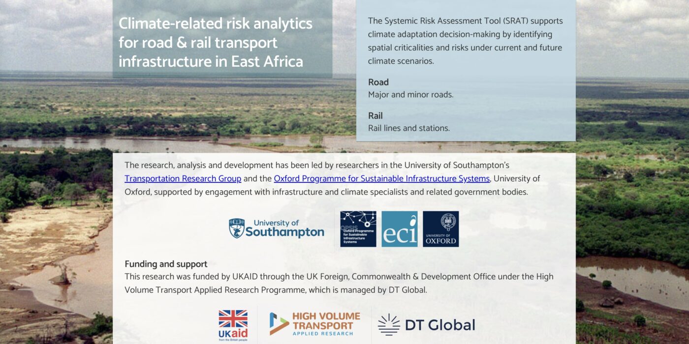
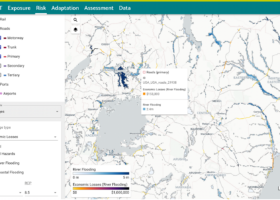
It provides an overview of the research findings underpinning the decision support tool which has been developed during the project. The decision support system is built around an interactive web platform and aims to support investment decisions and option selection for long distance strategic land transport networks exposed to climate risks. It is the first multi-state transport infrastructure decision support system in a low-income country context, based on a case study region covering Uganda, Zambia, Kenya and Tanzania, and is freely available online.
The underlying research has focused on developing a range of future background scenarios for transport development in the case study region, identifying and assembling datasets which form the basis for an assessment of transport resilience and sustainability. Data requirements, methodologies, related frameworks and example results for the underlying research are presented throughout the report, which also summarises the development of the decision support tool and provides case study examples based on potential future road transport project and policy interventions in the case study region. The case studies were identified in discussions during stakeholder workshops.
Details of the three sets of online workshops held during the project are provided, as well as an overview of the four in-country demonstration workshops carried out in September 2022. A summary report is available separately.
Publications with the same themes


Publications with the same study countries
Related news & events
News
Blog

Blog
News

Blog

Blog
PDF content (text-only)
Month Year Contract ref: Crown Agents ref: Final Report Decision support systems for resilient strategic transport networks in low-income countries January 2023 Project HVT/043 Decision Support Systems for Resilient Strategic Transport Networks in Low Income Countries This research was funded by UKAID through the UK Foreign, Commonwealth & Development Office under the High Volume Transport Applied Research Programme, managed by DT Global (formerly IMC Worldwide). The views expressed in this report do not necessarily reflect the UK government's official policies. Reference No. HVT/043 Lead Organisation/ Consultant University of Southampton Partner Organisation(s)/ Consultant(s) University of Oxford Title Decision support systems for resilient strategic transport networks in low-income countries – Final report Type of document Report Theme Long distance transport Sub-theme Resilience and sustainability Author(s) Adrian Hickford, Simon Blainey, Raghav Pant, Diana Jaramillo, Tom Russell, John Preston, Jim Hall, Marcus Young, Gordon Glasgow Lead contact Simon Blainey Geographical Location(s) Southampton/Oxford, UK (Researchers) Kenya, Tanzania, Uganda, Zambia (Case study countries) Abstract This is the final technical report of project HVT043, "Decision Support Systems for Resilient Strategic Transport Networks in Low Income Countries". It provides an overview of the research findings underpinning the decision support tool which has been developed during the project. The decision support system is built around an interactive web platform and aims to support investment decisions and option selection for long distance strategic land transport networks exposed to climate risks. It is the first multi-state transport infrastructure decision support system in a low-income country context, based on a case study region covering Uganda, Zambia, Kenya and Tanzania, and is freely available online at https://east-africa.infrastructureresilience.org/. The underlying research has focused on developing a range of future background scenarios for transport development in the case study region, identifying and assembling datasets which form the basis for an assessment of transport resilience and sustainability. Data requirements, methodologies, related frameworks and example results for the underlying research are presented throughout the report, which also summarises the development of the decision support tool and provides case study examples based on potential future road transport project and policy interventions in the case study region. The case studies were identified in discussions during stakeholder workshops. Details of the three sets of online workshops held during the project are provided, as well as an overview of the four in-country demonstration workshops carried out in September 2022. A summary report is available separately. Keywords Long-distance transport; Risk and resilience; Sustainability; Sustainability indicators; Decision support systems Funding FCDO High Volume Transport Applied Research Programme iv CONTENTS Executive Summary xiv 1. Introduction 1 1.1 Background to the research 1 1.2 Research questions and methodology 2 1.3 Stakeholder engagement 3 1.4 Long-distance transport in LICs 3 2. Scenarios and transport interventions 6 2.1 Assessing trends and setting the baseline 6 2.2 Scenario and intervention components 7 2.3 Scenario and intervention generation 8 2.3.1 Generation methodology 8 3. Data review and assembly 11 3.1 Environmental data assembly 12 3.1.1 Climate data 12 3.1.2 Flood hazard data 12 3.1.3 Other hazard data 14 3.2 Transport network location and topology data 14 3.2.1 Road network topology and road properties 15 3.2.2 Railways network topology 18 3.2.3 Ports and inland waterways 21 3.2.4 Airports 22 3.3 Data on vehicles 23 3.3.1 Road vehicle fleet 23 3.4 Data on socio-economic drivers of transport demand 24 3.4.1 National population change 24 3.4.2 Sub-national population change – regional trends and urbanisation 25 3.4.3 Economic change 26 3.4.4 Transport costs 26 3.5 Data for future scenarios and potential interventions 26 3.5.1 Exogenous drivers of demand 27 3.5.2 Vehicle and network use 29 3.5.3 Policy and planning 30 3.5.4 Impact of Covid-19 and other health related issues 33 3.6 Direct damage assessment data 34 3.6.1 Flood fragility curves 34 3.6.2 Rehabilitation costs 35 3.7 Infrastructure network flow data 36 3.7.1 Global trade flows between countries 36 3.7.2 Allocation of trade flows to airports and ports 38 3.7.3 Identifying locations on road networks for flow disaggregation 39 3.7.4 Flow allocation along routes 40 3.7.5 Projecting flows to the future 42 3.7.6 Flow results 43 v 3.8 Adaptation options data 46 3.9 Data review summary 48 4. Development of the tool 49 4.1 User interface 49 4.1.1 Introduction 49 4.1.2 Exposure 50 4.1.3 Risk 52 4.1.4 Adaptation 53 4.1.5 Sustainability assessment 54 4.1.6 Data 54 4.2 Architecture 54 4.2.1 Database 55 4.2.2 API server 57 4.2.3 Vector tile server 59 4.2.4 Raster tile server 60 4.2.5 Gateway 60 4.2.6 Frontend 60 4.3 Access to the tool 60 4.4 Code availability 60 5. Transport risk and adaptation analysis 61 5.1 Introduction 61 5.1.1 Research approach 62 5.2 Methodology for transport risk and adaptation analysis 63 5.2.1 Overview 63 5.2.2 Methodological framework for risk assessment 64 5.2.3 Adaptation assessment and estimation 66 5.2.4 Summary of output metrics 68 5.2.5 Wider application of the methodology 68 5.2.6 Interpretation of the models and results for risk and adaptation decision-making 69 5.3 Risk and adaptation analysis and results 70 5.3.1 Flood exposure analysis 70 5.3.2 Direct damage estimates 72 5.3.3 Expected annual damages 74 5.3.4 Expected annual economic losses 78 5.3.5 Adaptation assessment 82 5.3.6 Sensitivity analysis 88 5.4 Risk and adaptation analysis conclusions 95 6. Sustainability indicators and option assessment tool 96 6.1 Introduction 96 6.1.1 Sustainable transport and LDT 96 6.2 Sustainable Development Goals and LDT 97 6.3 Development of sustainable transport indicators for LDT 100 6.3.1 Identification and quantification of indicators 101 6.4 Developing a methodology for the option assessment tool 105 6.4.1 Generating comparative results using a decision matrix 107 vi 6.5 Impacts of change on sustainability indicators 108 6.5.1 Interactions between sustainability indicators 109 6.5.2 Interventions and their impact on sustainability indicators 111 6.5.3 Exogenous scenarios and their impact on sustainability indicators 112 6.5.4 Generating values for the option assessment tool 113 6.6 A worked example 117 6.7 Sustainability indicators and option assessment tool conclusion 120 7. Stakeholder engagement and impact 121 7.1 Online workshops 121 7.2 In-country workshops 121 8. Case Study examples 125 8.1 Uganda: road expansion project 125 8.2 Kenya: long-distance highway projects 126 8.3 Zambia: impact of transport emissions standards 129 8.4 Tanzania: focus on rail sector upgrades 130 8.5 Pan-regional: effects of flooding near border crossings 131 9. Conclusions and next steps 133 9.1 Conclusions 133 9.2 Summary of dissemination activities 135 9.3 Next Steps 135 Bibliography 137 Appendix A: Risk and adaptation analysis extended results 150 A.1 Coastal flooding results 150 A.2 Freight flow results 151 A.3 Expected annual damages results 153 A.4 Expected annual losses results 159 A.5 Sensitivity results 165 Appendix B: Online survey and elicitation of expert knowledge 169 Appendix C: Sustainability indicators – related studies 177 EAST (Early Analysis and Sifting Tool) 177 SuM4All (Sustainable Mobility for All) 178 TERM (Transport and Environment Reporting Mechanism) 179 ELASTIC (Evaluative and Logical Approach to Sustainable Transport Indicator Compilation) 181 STAR (Sustainability Tool for the Appraisal of Road projects) 181 Other studies 182 Appendix D: Sustainability indicators in context of scenarios and interventions 184 Appendix E: Examples of different approaches to the sustainability assessment 193 vii TABLES Table 1: Key data for trend and baseline generation............................................................................................ 7 Table 2: Description of open-source flood datasets used in this study .............................................................. 13 Table 3: Estimated kilometres of paved and unpaved roads for case study countries derived from 2021 OSM data...................................................................................................................................................................... 16 Table 4: National road networks, case study countries...................................................................................... 17 Table 5: Details of the railway networks classified by their status of use, gauge width and length in each country................................................................................................................................................................. 20 Table 6: List of maritime and inland waterway ports included in the study....................................................... 22 Table 7: List of airports of significance in the case study countries with their annual imported and exported freight tonnages .................................................................................................................................................. 22 Table 8: Vehicle fleet composition, case study countries................................................................................... 24 Table 9: Regional population in Kenya (Source: Kenya Census and citypopulation.de) ..................................... 25 Table 10: Measures and outcomes in East Africa (from World Bank AICD Research)........................................ 29 Table 11: Asset level rehabilitation/construction cost information used for estimating direct damages.......... 35 Table 12: Allocation of UNCTAD commodity sectors to macroeconomic sectors that generate the commodities for exports and that receive commodities as imports in case study countries .................................................. 37 Table 13: Description of socio-economic datasets used for disaggregating economic activity and assigning it to nearest road nodes in Africa and HVT specific countries.................................................................................... 40 Table 14: Estimates of the values of the parameters in the generalised cost function for transport flow allocation ............................................................................................................................................................. 41 Table 15: Flow capacities in tonnes/days assigned to rail and road links for transport flow allocation............. 42 Table 16: Impact of adaptation options on damage curves and high frequency cut-offs.................................. 46 Table 17: Description of adaptation options considered with costs, visual examples, and relevant assets ...... 47 Table 18: Features table schema......................................................................................................................... 55 Table 19: Expected damages table schema......................................................................................................... 55 Table 20: Return period damages table schema................................................................................................. 56 Table 21: Adaptation costs and benefits table schema....................................................................................... 56 Table 22: Overview of metrics produced from the analysis................................................................................ 68 Table 23: List of identified ports and airports with their hazard exposure scenario results .............................. 72 Table 24: Mean expected annual damages to railways and roads in million US$ from fluvial and coastal flooding under baseline conditions and for future outlooks under RCP 4.5 and 8.5.......................................... 74 Table 25: Example of adaptation CBA results for a sample rail asset showing the effectiveness of each option considered for this asset. The most preferred option is the flood wall, which is highlighted in the table......... 82 Table 26: Input parameters chosen for global sensitivity analysis...................................................................... 88 Table 27: Comparison of reviews of transport's impact on SDGs....................................................................... 98 Table 28: SDG targets which are directly influenced by LDT............................................................................... 99 Table 29: Framework of component themes of sustainable transport ............................................................ 101 Table 30: Indicators selected for inclusion in the study)................................................................................... 102 Table 31: Example decision matrix for Environmental indicators, no weightings............................................ 107 viii Table 32: Example decision matrix for Environmental indicators, with higher weightings assigned to emissions and energy consumption................................................................................................................................... 108 Table 33: Example decision matrix for Environmental indicators, with higher weightings assigned to emissions and energy consumption, and lower multipliers assigned as appropriate ....................................................... 108 Table 34: Interactions between Environmental and other sustainability indicators........................................ 109 Table 35: Interactions between Economic and other sustainability indicators................................................ 109 Table 36: Interactions between Social and other sustainability indicators ...................................................... 111 Table 37: Interactions between intervention types and sustainability indicators............................................ 111 Table 38: Interactions between exogenous scenarios and sustainability indicators........................................ 113 Table 39: Pre-set values for Option 1: Infrastructure construction, and subsequent user inputs.................... 118 Table 40: Pre-set values for Option 2: Infrastructure maintenance, and subsequent user inputs................... 119 Table 41: Pre-set values for Option 3: Infrastructure construction and maintenance combined, and user inputs ........................................................................................................................................................................... 119 Table 42: In-country workshops summary ........................................................................................................ 122 Table 43: Case study 1 – Default and revised values for impacts and weightings of related sustainability indicators........................................................................................................................................................... 126 Table 44: Case study 2 – Estimated direct damages......................................................................................... 127 Table 45: Case study 2 – Expected indirect losses per day (most affected road segments)............................. 128 Table 46: Case study 2 – Default and revised values for impacts and weightings of related sustainability indicators........................................................................................................................................................... 129 Table 47: Case study 3 – Default and revised values for impacts and weightings of related sustainability indicators........................................................................................................................................................... 129 Table 48: Case study 4 – Default and revised values for impacts and weightings of related sustainability indicators........................................................................................................................................................... 131 Table 49: Case study 5 – Default and revised values for impacts and weightings of related sustainability indicators........................................................................................................................................................... 132 FIGURES Figure 1: Case study region 2 Figure 2: Work programme structure 3 Figure 3: Example of a generic long-distance transport network 4 Figure 4: Generic LDT network applicable to this study 4 Figure 5: Trend and baseline data framework 6 Figure 6: Summary of components within each scenario or intervention theme 8 Figure 7: Schematic view of generation of future transport interventions and scenarios 9 Figure 8: Example of intervention settings for vehicle and network use theme 9 Figure 9: Example of intervention settings for policy and planning theme 10 Figure 10: Example of scenario generation for exogenous drivers of demand 10 Figure 11: Average monthly climate data (Source: World Bank Climate Change Knowledge Portal) 12 ix Figure 12: Map visualisation of sample river flood maps showing areas flooded and their flood depths for a 1/1,000 return period under (a) baseline conditions and (b) in 2080 under RCP 8.5 climate scenario 14 Figure 13: Map representation of the OSM road network created for this study showing roads classified as (a) trunk, primary, secondary, and tertiary; and (b) paved or unpaved 16 Figure 14: Road quality index (World Economic Forum) 18 Figure 15: Map representation of the data created for the study showing the status of existing and proposed spatial railway routes across Kenya, Tanzania, Uganda and Zambia 20 Figure 16: Map representation of all the ports considered in the study 21 Figure 17: Map representation of the airports considered in the study with their annual imported and exported freight tonnages 23 Figure 18: Population trends (World Bank data) 24 Figure 19: Urbanisation trends (World Bank data) 25 Figure 20: Economic trends, GDP (World Bank data) 26 Figure 21: Fuel prices at pump (World Bank and IEA data) 26 Figure 22: Population projections (UN DESA) 27 Figure 23: A range of GDP future scenarios for the case study countries 28 Figure 24: Mobile phone subscriptions per 100 people (World Bank data) 30 Figure 25: Kenyan imports and exports (in Kenyan Shillings) 2011-2021 (Source: Kenya National Bureau of Statistics, Leading Economic Indicators) 33 Figure 26: Example profiles of economic recovery after pandemic (full medium-term recovery in red, partial recovery in orange) 34 Figure 27: Generalised direct damage (fragility) curves vs flood depths for different types of infrastructure assets (a) paved roads; (b) unpaved road; (c) railway lines. 35 Figure 28: Visual representation of (a) the trade shipping costs to Free on Board (FOB) in US$ for one commodity being traded between Tanzania and rest of the world (source: unctadSTAT website); and (b) ODmatrices for the study derived from the global data 37 Figure 29: Volume of export-import tonnage being shipped in 2015 between countries and the Port of Mombasa in Kenya and the Port of Dar es Salaam in Tanzania (all estimates are from statistics compiled by the Kenya Port Authority and the Tanzania Port Authority annual reports) 39 Figure 30: Road freight flows in value (US$) per day for (a) baseline year 2019, (b) 2030, (c) 2050, and (d) 2080 44 Figure 31: Railway freight flows in value (US$) per day for (a) baseline year 2019, (b) 2030, (c) 2050, and (d) 2080 45 Figure 32: SRAT home page 50 Figure 33: Asset exposure to river flooding 51 Figure 34: Expected direct damages from river flooding 52 Figure 35: Adaptation options 53 Figure 36: Sustainability assessment 54 Figure 37: Identify the road "KEN_KEN_roade_722142" in the graphical user interface 59 Figure 38: Graphical representation of a multi-modal transport system-of-systems 63 Figure 39: Graphical representation of transport system-of-systems risk and adaptation assessment framework 66 x Figure 40: Graphical representation of the CBA analysis for evaluating the effectiveness of adaptation options 67 Figure 41: Length of flooded (a) roads and (b) railways from river flooding in 2030, 2050, and 2080 under baseline, RCP 4.5, and RCP 8.5 scenarios 71 Figure 42: Direct damages to (a) roads and (b) railways from river flooding in 2030, 2050, and 2080 under baseline, RCP 4.5, and RCP 8.5 scenarios 73 Figure 43: Mean expected annual damages to railways and roads in million US$ from fluvial and coastal flooding under baseline conditions and for future outlooks under RCP 4.5 and 8.5 74 Figure 44: Expected annual damages to roads and from river flooding under (a) baseline conditions and for 2080 under (b) RCP 4.5 and (c) RCP 8.5 76 Figure 45: Expected annual damages to railways from river flooding under (a) baseline conditions and for 2080 under (b) RCP 4.5 and (c) RCP 8.5 77 Figure 46: Mean expected annual losses per day of disruption to roads and from river flooding under (a) baseline conditions and for 2080 under (b) RCP 4.5 and (c) RCP 8.5 79 Figure 47: Mean expected annual losses per day of disruption to railways from river flooding under (a) baseline conditions and for 2080 under (b) RCP 4.5 and (c) RCP 8.5 80 Figure 48: Mean EAD and EAEL under disruption durations of 15, 30, and 60 days for (a) road, and (b) rail assets ranked by assets with total risks greater than US$ 100,000 81 Figure 49: Maximum (a) benefit, (b) investment, and (c) BCR for adaptation options to roads 84 Figure 50: Maximum (a) benefit, (b) investment, and (c) BCR for adaptation options to railways 85 Figure 51: BCR ranges of roads for (a) Swales; (b) Spillways; (c) Mobile flood embankments; (d) Flood wall; (e) Drainage rehabilitation; and (f) Upgrading to paved under RCP 4.5 and 8.5 86 Figure 52: BCR ranges of railways for (a) Swales; (b) Spillways; (c) Mobile flood embankments; and (d) Flood wall under RCP 4.5 and 8.5 87 Figure 53: First-order and second-order sensitivity index values showing influence of input parameters on river flooding induced direct damage and indirect economic loss estimates for roads 89 Figure 54: First-order and second-order sensitivity index values showing influence of input parameters on coastal flooding induced direct damage and indirect economic loss estimates for roads 90 Figure 55: First-order and second-order sensitivity index values showing influence of input parameters on river flooding induced direct damage and indirect economic loss estimates for rail 91 Figure 56: Influence of variables on different adaptation options for river flooding of roads 93 Figure 57: Influence of variables on different adaptation options for river flooding of railways 94 Figure 58: Simplified methodology for the option assessment tool 106 Figure 59: Example decision matrix for all interventions, scenarios and indicators 114 Figure 60: Example screenshot setting out intervention selection for Option 1 117 Figure 61: Example screenshots changing values for 'Habitat and ecosystem disruption' multiplier and 'Density of transport networks' weighting for Option 1 118 Figure 62: Example screen presenting summary results for Option 1 119 Figure 63: Case study 1 – Uganda's Busega-Mpigi expressway, flood risk assessment 125 Figure 64: Case study 2 – Kenya's Lesseru-Kitale and Morpus-Lokichar road improvements, flood risk assessment 127 Figure 65: Case study 2 – Estimated annual damages chart 128 Figure 66: Case study 4 – Tanzanian rail construction, flood risk assessment 130 xi Figure 67: Case study 5 – Flood risk at border crossings between Zambia and Mozambique 132 ABBREVIATIONS and ACRONYMS AfDB African Development Bank AICD Africa Infrastructure Country Diagnostic AIDI Africa Infrastructure Development Index API Application Programming Interface BaU / B-a-U Business as Usual BCR Benefit-Cost Ratio CBA Cost-Benefit Analysis CCTTFA Central Corridor Transit Transport Facilitation Agency CIA Central Intelligence Agency CO2 Carbon dioxide COG Cloud-Optimised GeoTIFF COMESA Common Market for Eastern and Southern Africa DPSIR Driving force, Pressure, State, Impact, and Response DRC Democratic Republic of Congo EAC East African Community EAD Expected Annual Damages EAEL Expected Annual Economic Losses ECON Economic Indicators EEA European Environment Agency ELASTIC Evaluative and Logical Approach to Sustainable Transport Indicator ENV Compilation Environmental Indicators ESCAP Economic and Social Commission for Asia and the Pacific EU European Union GC Generalised cost GCM Global Climate Model GDP Gross Domestic Product GIS Geographical Information Systems GPS Global Positioning System GVA Gross Value Added FCDO Foreign, Commonwealth & Development Office FCFA Future Climate for Africa FEAFFA Federation of East African Freight Forwarders Associations FOB Free-on-board GCA Global Center on Adaptation GFEI Global Fuel Economy Initiative GHG Greenhouse gas GRA Global Roadmap of Action gROADS Global Roads Open Access Data Set HGV Heavy goods vehicle HTTP HyperText Transfer Protocol HVT High Volume Transport IEA International Energy Agency IFPRI International Food Policy Research Institute IPCC Intergovernmental Panel on Climate Change xii IRI International Roughness Index JSON JavaScript Object Notation KeNHA Kenya National Highways Authority km kilometre KPA Kenya Ports Authority ktCO2e kilotonnes of carbon dioxide equivalent LDT Long-distance transport LGV Light goods vehicle LIC Low-income country LMIC Lower middle-income country MCA Multi-Criteria Analysis mm millimetres MVT Mapbox Vector Tile NASA National Aeronautics and Space Administration NPV Net Present Value OD Origin-Destination OSM Open Street Map PCU Passenger car unit PGA Peak Ground Acceleration PIDA Programme for Infrastructure Development in Africa pkm passenger kilometres PM2.5 Particulate matter (two and one half microns or less in width) PNG Portable Network Graphics RCP Representative Concentration Pathway RDA Road Development Agency (Zambia) RFID Radio-Frequency Identification ROCKS Road Costs Knowledge System RQ Research question SDG Sustainable Development Goal SGR Standard gauge railway SLOCAT Partnership on Sustainable, Low Carbon Transport SOC Social Indicators SRAT Systemic Risk Assessment Tool SSL Secure Socket Layer STAR Sustainability Tool for the Appraisal of Road projects SuM4All Sustainable Mobility for All TANROADS Tanzania National Roads Agency TERM Transport and Environment Reporting Mechanism tkm tonne kilometres TPA Tanzania Ports Authority TTTFP Tripartite Transport and Transit Facilitation Programme vkm Vehicle kilometres UK United Kingdom UN United Nations UNCTAD UN Conference on Trade And Development UN DESA United Nations Department of Economic and Social Affairs UNDP United Nations Development Programme UNRA Uganda National Roads Authority xiii US United States USD US Dollars VTPI Victoria Transport Policy Institute WEF World Economic Forum WHO World Health Organisation WP Work Package xiv Executive Summary This report sets out the research undertaken during High Volume Transport Project (HVT) 043, 'Decision Support Systems for Resilient Strategic Transport Networks in Low Income Countries'. The HVT programme's overall aim is to strengthen the evidence base available to transport decision makers, helping them make investment decisions that enable high-volume road and rail transport to be greener, more accessible, more Overview This report highlights the first multi-state transport infrastructure decision support system in a lowincome country context, based on a case study region covering Uganda, Zambia, Kenya and Tanzania, freely available online at https://east-africa.infrastructureresilience.org/. The decision support system is built around an interactive web platform and aims to support investment decisions and option selection for long distance strategic land transport networks exposed to climate risks. The underlying research has focused on developing a range of future background scenarios for transport development in the case study region, identifying and assembling datasets which form the basis for an assessment of transport resilience and sustainability. From the outset, the project has focused on four specific research areas: • Future scenarios and transport interventions A framework has been created to help classify relevant transport intervention types which affect the use and nature of long-distance transport networks, and guide the development of exogenous scenarios of change in demand related to population growth, economic factors and climate change. • Data review and assembly Beyond the data associated with scenarios and transport interventions, the risk and resilience aspect of the decision support tool requires data on transport network topology and use, in order to map out where climate hazards are greatest, where they overlap with transport assets, and the impact and costs of any disruptions caused by flooding. • Climate resilience of road and rail networks A system-of-systems assessment of climate risk and adaptation options has been developed, focusing on four main themes: Criticality (the importance of a transport link based on its disruptive impact on the wider network); Vulnerability (understanding the negative consequences caused by failures of transport links from external shock events); Risk (the likelihood of hazards occurring, and the subsequent consequences of transport link failures); and Adaptation planning (identifying which assets and locations should be prioritised for targeted investments to provide maximum benefits in reducing risks. Results suggest that considerable lengths of roads and railways are currently exposed to river flooding, and there is a significant increase in the exposure lengths when comparing the future climate scenario driven flood outcomes with the current situation. • Sustainability assessment The option assessment tool is based on a range of sustainability indicators, grouped around the three main 'pillars' of sustainability: environmental, economic and social sustainability, and can compare the impacts of future scenario change and transport interventions aimed at improving long-distance transport, either by technological advances, government policy or transport planning. Stakeholder engagement has been key to this research, and ongoing partnerships with relevant organisations in each of the four case study countries have been crucial in identifying a range of multisectoral stakeholders who could provide feedback on the research. Firstly, three rounds of online workshops each focused on a different aspect of the research. Secondly, a set of in-person workshops in each of the case study countries covered each aspect of the project, and demonstrated an early version of the web-based decision support tool. Finally, five potential case studies were identified during the incountry workshops, and feedback from the workshop discussions has helped in the further development of the online tool and the case studies. xv affordable, more inclusive and safer, and has the overarching goal of increasing access in low-income countries to affordable transport services, more efficient trade routes and safer, low carbon transport. Focusing on the original HVT theme of climate change adaptation and mitigation, this project supports investment decisions and option selection for long distance strategic land transport networks exposed to climate risks by creating the first multi-state transport infrastructure decision support system in a LIC context, based on a case study region covering Kenya, Tanzania, Uganda and Zambia. The decision support system is built around an interactive web platform which is freely and openly available online at https://eastafrica.infrastructureresilience.org/. The tool has been created based on research undertaken at the Universities of Southampton and Oxford, in collaboration with stakeholder partners in each of the case study countries. From the outset, the project has aimed to answer four Research Questions, which are set out below, together with a summary of how this research has sought to answer each. They have been investigated through a series of six linked Work Packages (WP), as shown below; the research findings from WP1 to WP4 map on to the research questions RQ1 to RQ4 respectively. These research questions have been considered within the context of long-distance transport, which is defined as being the movement of goods and people between some generator or attractor hub, such as a major port or airport, and major destinations along a series of corridors emanating from that hub. For the purposes of this study, the components of long-distance transport are the physical transport networks (mainly roads and railways, along with inland waterways) that facilitate movement, and the vehicles which use these networks to move goods and people (predominantly freight traffic and passenger rail). RQ1: What is the expected range of future scenarios for transport development in the case study region, with respect to factors such as population, economic growth, climate and technology? One of the main aims of this research project was to undertake analysis of the potential effectiveness and consequences of transport system interventions in LICs, and for this to be achieved it is necessary to have information on the exogenous conditions in which the interventions might be situated, along with an understanding of the different types of potential transport interventions. WP1 of this project focused on the production of a framework to classify intervention types and guide the development of exogenous scenarios. Before building this framework, an assessment of change and trends between 2000 and 2018 was undertaken, which not only provided an understanding of the likely future trajectories of change for relevant factors based on historical trends, but also provided insight into the availability, reliability and accuracy of data related to long-distance transport networks. The trend assessment highlighted the three different types of factors which would need to be included as inputs to the decision support tool: i. Exogenous factors – drivers of demand such as population growth, economic factors such as GDP and energy costs, and climate change. xvi ii. Transport-related change – intervention factors which are largely outside the control of transport policy makers in LICs, such as changes in vehicle, fuel and other technologies, and behaviour change affecting how long-distance transport networks are used. iii. Future transport policy and strategic interventions – endogenous factors derived from existing plans to improve the long-distance transport network, or strategies for changing how the networks are currently used. In order to generate future options for each of these components, it is possible to use established datasets and projections where they exist, such as for future population change (UN DESA), and global climate change (IPCC and Future Climate for Africa). Historical trends can also be used to provide an estimate of future change where good quantitative data exists, such as for GDP, and simple modifications to these future estimates can provide higher or lower rates of change, reflecting the uncertain nature of future scenario development. However, for many of the transport-related components of future change, such reliable datasets do not exist. In that case, it is possible to consider more qualitatively how those components are likely to affect either the transport networks, the origin-destination matrix of people and goods, or the costs associated with long-distance transport. A combination of these approaches has been used in this project to provide an understanding of the likely impacts of future change, and the framework developed in WP1 provides a method of generating a range of exogenous scenarios and a classification of different intervention types most likely to impact the use and nature of long-distance transport networks in the future. RQ2: What data are required in order to develop an effective decision support system for long distance transport in LICs? While the data gathering exercise undertaken as part of WP1 provided an understanding of the impact of exogenous drivers of change and possible transport interventions, the risk and resilience aspect of the decision support tool also required more detailed data on transport network topology, flows and movements of goods and people. This was the focus of WP2, which initially set out the data requirements for the risk analysis work to be undertaken, and subsequently reviewed and assembled relevant open-source datasets. This project uses river (fluvial) and coastal flood maps (openly available from the Aqueduct flood product datasets) to estimate climate risks to transport assets, by generating flood return period extents and flood depths for flooding across the case study countries. The resultant future flood maps can then be used in the decision support tool to identify locations or transport assets that would be at risk of damage caused by different flood scenarios, with outputs given for the years 2030, 2050, and 2080, for a range of different flooding extents under climate change scenarios represented by different Representative Concentration Pathways (RCP 4.5 and RCP 8.5). In order for this flood analysis and subsequent damage costs estimation to be undertaken, the decision support tool requires a detailed model of the different infrastructure networks and associated assets, along with an estimate of the network flows. There are a range of data collection requirements for creating infrastructure network models with flows. Physical topological network information describes the network structure, and the existence of physical links with information about their connecting node locations is a necessary and essential condition for the creation of transport network models, because of the geospatial nature of the transport systems. Network condition attributes such as link length, link width and link condition help to provide details of the physical network properties, used to infer their intersections with hazards and failure criteria. Network cost assignment attributes provide the basis of selecting the least generalised cost route (an estimate of the monetary value in US Dollars of transporting freight) between a selected origin-destination pair and modal option, in order to assign origin-destination flows on the networks. Data for the road networks (classified as motorways and trunk roads, primary roads, secondary roads, and tertiary roads in this project) and rail networks (classified as functional (the railway routes which were in operation) and non-functional (the railway routes which were no longer in use, or were being rehabilitated following periods of disuse)) were extracted from OpenStreetMap, which provides very accurate location, geometry and connectivity information for long-distance transport. The rail network data was enhanced to incorporate missing information, for example with regard to the location of some stations. xvii Ports are significant hubs linking to the road and railway networks. The waterway ports are either maritime ports located along the eastern coastline of the region, connecting it to the routes on the Indian Ocean, or inland ports which tend to be concentrated along two main lake waterbodies (Lake Victoria, where the ports connect Tanzania to other ports in Uganda and Kenya, and Lake Tanganyika, where the ports connect Tanzania to other ports in Burundi, The Democratic Republic of Congo and Zambia). Data on these ports is not readily available in global open access datasets, but can be extracted from national port authority documents and annual reports. The project also considers the main airports in the case study countries, with significant volumes of freight or passengers that would have an effect on the long-distance land transport networks. The largest airport in the case study region is in Nairobi (Jomo Kenyatta International Airport, Kenya), with other large airport hubs located in Kampala (Entebbe International Airport, Uganda), Dar Es Salaam (Julius Nyerere International Airport, Tanzania), Lusaka (Kenneth Kaunda International Airport, Zambia), Eldoret (Eldoret international Airport, Kenya) and Mombasa (Moi International Airport, Kenya). Data on annual passenger movements and imported and exported freight tonnage can be extracted from country specific reports. A significant challenge that has been faced in this project is the lack of any information on network flows in terms of passenger or freight movements along road and rail links, with no openly available road or rail passenger or freight traffic flow model or data available for Africa or the case study countries. There are, however, global datasets from which estimates can be created of trade import-export flows between countries, using high-level statistics at specific border crossings (ports, airports) to assign flows to specific locations in countries. Modal-splits are estimated to assign flows to road and rail networks and then assigning flows along networks based on the conglomeration of population and economic activities within countries. Beyond the topological and flow data essential to traffic network flow models, and the intersection of those networks with flood maps, further data is required on the impacts of flooding on the various transport assets, in order to assess the likelihood of damage, and the subsequent direct and indirect costs of network disruptions. Flood fragility curves are used to estimate the amount of damage an asset would sustain due to hazard exposures, while a range of estimated rehabilitation or reconstruction costs for railway lines and for different types of paved or unpaved roads are derived from multiple sources, providing an understanding of the typical costs of major construction projects, and the variability of such costs. These data can be combined to generate estimated direct and indirect costs caused by flooding, but for costbenefit analyses to be undertaken, further information is required on the costs and likely impacts on flood defence of the array of strategies and measures that are available and appropriate. These strategies and measures are referred to here as 'adaptation options' for sections of roads and railway tracks. The six different adaptation options considered are: swales (broad shallow channels topped with vegetation, designed to attenuate and infiltrate runoff volume from adjacent impervious surfaces), spillways (designed to discharge flows that cannot either be used immediately or stored in a reservoir for future use), mobile flood embankments (mobile and reusable inflatable tube segments that are used to insulate/dam flood water, offering immediate use and protection, and subsequent storage), flood wall (a freestanding, permanent, engineered structure designed to prevent encroachment of floodwater), drainage rehabilitation (the systematic removal of accumulated material from watercourses, canals, or drainage systems, increasing the efficient conveyance of water), and upgrading unpaved roads to paved. The actual costs and the applicability of each option will depend heavily on the specific local conditions and topography. For example, the implementation of swales may be constricted by space and slope considerations as well as by suitability of native vegetation. RQ3: How resilient is long distance transport infrastructure in the case study region to climate-related and other hazards? Using the data set out above, the research approach adopted in this study is one that (i) maps out where climate hazards are greatest; (ii) identifies the elements and locations in the transport network that are exposed to climate hazards; (iii) assesses the significance of climate risk by mapping the flows of people and goods on the network and the potential for socio-economic disruption; (iv) assesses the costs and benefits (in terms of risk reduction) of adaptation options under different future scenarios; and (v) prioritises adaptation options, so that limited budgets can be used to climate-proof the network as efficiently as possible. xviii A methodological framework for climate risk and adaptation assessment has been developed and implemented for multi-modal infrastructure systems comprised of the road and rail networks, and the airports and waterway ports that connect with these networks. The road and rail networks are large-scale spatially distributed systems with complex interactions, each defined as a collection of nodes joined together by a collection of links. Nodes are point representations of key locations of physical facilities and human systems in the transport systems – ports, airports, railway stations, and road junctions. Links are line representations of physical connections between nodes – road sections, railway lines, and waterway routes. The multi-modal transport system-of-systems is subsequently a networkof-networks. The framework presents different types of system-of-systems assessments useful for decision-making: 1. Criticality assessment – measuring the importance of a transport link based on its disruptive impact on the rest of the transport infrastructure. 2. Vulnerability assessment – measuring of the negative consequences due to failures of transport links from external shock events, carried out in the context of natural hazards and resulting in understanding of the relative impacts of hazards on the continued transport availability. 3. Risk assessment – providing an understanding of the likelihood of hazards occurring, and the subsequent consequences of transport link failures. 4. Adaptation planning – identifying which assets and locations should be prioritised for targeted investments to provide maximum benefits in reducing risks. Within the framework the steps of network risk estimation are divided into two parts: 1. Direct damage calculations – losses that are incurred due to the physical damages to the network nodes and links, when they are exposed to extreme hazards (i.e. flooding in this case). 2. Indirect economic loss calculations – losses that are incurred due to disruptions to network flows following direct damage to network nodes and links. In this study, such losses are estimated in terms of changes to the freight flows on these networks, but similar methods could be extended to estimating changes to passenger flows. In particular freight flow disruptions either lead to increased costs of rerouting and redistributing freight along networks, or loss of value of freight when there are no flow rerouting options, especially if the damaged nodes or links only connected to a single location on the network. The system-of-systems methodological approach consists of the following components: • Hazard assembly – external shock events which initiate failure in the transport systems, quantified through static hazard maps that capture the spatial extent, magnitude, return period or the annual exceedance probability, climate scenario and time epoch. • Multi-modal transport networks assembly – achieved by collecting geospatial data for use in Geographical Information Systems (GIS) and creating connected network models, identifying and assigning attributes to locations on the networks, identifying key nodes of freight transport origins and destinations, integrating freight data with the network locations, and assigning origin-destination flows onto the networks based on a least generalised cost criteria to create flow estimates. • Exposure analysis – achieved by creating spatial intersections of hazards and network assets, overlaying each hazard map layer with each asset geometry and estimating the magnitude of the hazard at a particular location, and the extent of the asset geometries that are within the hazard areas. The process results in compiling hazard levels and spatial extents affecting each infrastructure asset across all return periods, climate scenarios, and time epoch of every hazard type. This leads towards the estimation of direct and indirect risks associated with assets and network failures. • Direct damage estimation – quantifying the rehabilitation costs (in US$) of assets subjected to different hazard shocks across current and future climate scenarios. This is achieved by selecting a level of hazard that might cause physical damage to assets such that there will be a need for rehabilitation, then using fragility or vulnerability functions which quantify the percentage (or fraction) of replacement cost xix sustained by an asset for a given magnitude of a hazard. In the analysis, the uncertainties of vulnerability functions and asset unit costs are combined to quantify a range of direct damage costs to assets exposed to hazards. • Indirect economic loss estimation – measuring the disruptions to infrastructure networks' overall performance and services, in particular the indirect economic losses from import-export trade flow disruptions (in US$/day). This is achieved by identifying all existing origin-destination trade routes which are disrupted, rerouting flows towards alternative routes, and estimating flow disruptions in terms of freight tonnage lost when there are no rerouting options. • Direct and indirect risk metrics – estimated as a function of the hazard annual exceedance probabilities and the total impacts (direct damages plus indirect losses). Due to the uncertainties associated with hazards events and climate scenarios, asset fragilities, and disruption impacts, two risk metrics are estimated: a. Expected Annual Damage (EAD) – the average damage costs (US$) incurred for an asset in any given year due to a given hazard type for a given time epoch and climate scenario. b. Expected Annual Economic Losses (EAEL) – the average economic losses (in US$) incurred following the damages to an asset in any given year due to a given hazard type for a given time epoch and climate scenario. The asset level total risk can be calculated as total risk = EAD + EAEL. There are different ways in which the risk estimates can be presented, either through damage(loss)-probability curves or as a network map highlighting the most critical assets across the country in terms of value of EAD and EAEL estimates. This approach can be used to understand future transport failures and losses, by (a) assembling statistics on future origin-destination flow growth scenarios (based on different indicators such as projected trade growth, projected increase in tonnage growth at specific locations such as ports, airports); (b) incorporating structural changes to the networks (if possible) in terms of changing conditions of links; (c) estimating the changes in performance measures that determine new estimates for generalised cost functions in the future, and (d) creating modal options for new flow assignments. Once the estimation of asset level risks across multiple hazards, climate scenarios and time epochs is completed, an adaptation assessment with respect to a set of adaptation options can be undertaken, quantifying the effectiveness of different adaption options with estimated costs for building resilience (to climate shocks) of individual assets and networks. This is achieved through a cost-benefit analysis of a chosen option, where the costs of an adaptation option are compared with the benefits due to reduced or avoided risks. The estimation of costs, risk reduction benefits and co-benefits of adaptation options leads towards prioritisation of investment interventions, which is achieved by evaluating different options and ranking them by their benefit-cost ratios. The report presents a series of results showing the degree to which transport assets in the four case study countries are exposed to extreme river and coastal flooding. This is followed by the quantification of direct damages for different flood return periods. The risks are then quantified in terms of the EAD values at the asset level and the aggregated sum for the whole region, which is an indicative of the magnitude of largescale disaster impacts. Following these analysis results, the indirect risk estimates are shown as the EAEL values at the asset level, which capture the systemic impact of each asset's disruption on network performance. Having shown the risk analysis results, the findings from the adaptation assessment are presented in terms of the benefits, costs and BCR values of adaptation options associated with assets. Finally, sensitivity analysis results show how the output metrics are sensitive to some of the model assumptions The results suggest that considerable lengths of roads and railways are currently exposed to river flooding, and there is a significant increase in the exposure lengths when comparing the future climate scenario driven flood outcomes with the baseline. In almost all cases, there is no flooding in a 1/2 return period for the baseline, but some flooding is seen at this return period in the future. In the baseline (current) scenario, an average of 1.0% (1,790km) by length of the current road networks and 1.5% (158km) by length of the current railway networks are exposed to river flooding across all flooding scenarios considered. In a 1/5 flooding scenario, 182km of roads are flooded (an estimated US$ 29 million in xx direct damages), which increases to 2,243km in a 1/100 scenario (US$ 412 million in direct damages) and in the most extreme case to 3,333km in a 1/1,000 flooding scenario (US$ 688 million estimated direct damages). Railway networks show less variability to different flooding scenarios. For a 1/5 flooding scenario, 24km of railways are flooded (resulting in estimated direct damages of US$ 3.4 million). This increases to 304km for a 1/1,000 flooding scenario (resulting in direct damages as much as US$ 216 million). There is no predicted coastal flooding of railways. Roads are less exposed to coastal flooding than river flooding with only 7.3km of roads exposed to coastal flooding across all baseline scenarios. These low estimates of coastal flood exposures might also be as a result of low infrastructure coverage over the coastal areas, along with a low prediction of flooding in the hazard datasets. Under future climate outlooks, the flood risk to roads and railways gets more severe across all return periods. On average across all return periods in 2080 under RCP 8.5, 1.6% (2,876km) by length of the road networks and 1.9% (200km) by length of the future railway networks are exposed to fluvial flooding. This means that on average by 2080 an extra 1,086km of roads will be exposed to extreme fluvial flooding, which is quite a significant increase of 60% from baseline flooding estimates. Under RCP 8.5, transport networks will be even more exposed to flooding as compared to RCP 4.5. For example, in a future 1/5 river flooding, 705km of roads are potentially going to be flooded in 2080 under RCP 4.5, which is a significant increase from the 182km of baseline flooding. This increases to 1,066km of flooded roads in 2080 under RCP 8.5, a 485% increase from baseline flooding. If, as is suggested in other research, assets in the region are generally designed for 1/10 to 1/50 flood levels, then any significant increase in flood exposure and severity at lower return periods will result in road and railway assets (designed against existing levels of flood return period) being unable to withstand future extremes. These results imply that direct damage costs to transport networks from flood exposure will be substantially magnified in the future due to climate change. The results of the EAD analysis provide an estimate of the annual cost if direct damages from all hazard probabilities and magnitudes were spread out equally over time, and these results can be mapped to reveal those transport links with especially high EADs. The results presented in this report reveal that several segments of the road network in the case study region have significant EAD which increase in the future across both climate scenarios, particularly around the Great Lakes, in the east to northeast in Kenya, and along the southern part of the Zambezi River in Zambia. In the baseline year, EAD can reach as much as US$ 2.4 million. In 2080 under RCP 8.5, this can reach as much as US$ 3.9 million. When these risks occur in locations where the road density is very low, this might result in loss of connectivity for network users if just a few of the high-risk roads were all damaged at the same time. High EAD values seen along linkages close to where the rail damages were also significant could create potential connectivity issues if both networks were flooded at the same time. High EAD values for the cross-border roads can potentially impact trade. One of the highest EAD railway links is in Tanzania along the Central Corridor, which is the main route for transporting commodities from the port of Dar es Salaam towards the Lake Victoria ports providing access to Uganda and Burundi. Some of the highest EAD railway links in the case study area under future years are along proposed routes. Specifically: the new SGR line connecting Mwanza to Isaka, Tabora, and Makutupora in Tanzania; the proposed Mtwara line in Tanzania; and the Chipata-TAZARA line in Zambia. Future flooding risks must be taken into consideration when constructing these proposed lines in order to avoid investment losses from future failures. These results of the adaptation assessment show a significant number of assets on the road network for which options such as drainage rehabilitation are most effective, while installing flood walls and swales are also effective options in many cases. From these results it is estimated that investing in adaptation of the top 20 most benefit-incurring road investments would amount to about US$ 9 million in adaption costs (net present value) against of benefits of about US$ 875 million in avoided risk (net present value). For railways, the results suggest that options such as swales, flood walls and mobile flood embankments are the most effective adaptation options. Several of these options should be applied to new railway lines such as the new standard gauge railway line along the Central Corridor in Tanzania where swales could help avoid potential risks. Investing in adaptation measures for rail assets ranked in the top 20 most benefit incurring rail xxi investments would amount to about US$ 92 million adaptation costs (net present value) and provide US$ 234 million in avoided risk (net present value) benefits. The adaptation analysis shows that most of the highest benefits and cost-effective investments are key linkages that facilitate trade flows across the whole networks. For such assets there is a very compelling case for investing in climate adaptation to improve systemic resilience of transport networks. Based on these results, it is possible to prioritise the assets and locations for building climate resilience, while having estimates of the scales of adaptation investment requirements. The risk analysis presented here is a high-level indicative assessment of transport systems and their exposures, damages, economic losses, risks and adaptation options assessment due to flooding, and can be used to identify a significant sample of assets and locations of potential risks, at the regional scale. These analyses should be used as a first-order screening of potential assets that require further detailed investigation, which should be carried out subsequently. RQ4: How can the sustainability of long-distance transport systems in the case study region be quantified and assessed? Investments in long-distance land transport networks can help drive regional and national development in low-income countries, but while such developments can contribute to economic growth, they often impact negatively on society and the environment, contrary to the ideals of sustainable development. There is no consistent definition of 'sustainable transport', particularly in the context of long-distance transport. There are, however, commonalities among the various definitions in the literature, and the definition of sustainable long-distance transport has been developed for this project as "a transport system that is compatible with net-zero emissions of greenhouse gases, has a net-neutral or net-positive impact on environments at all scales, provides safe and secure accessibility and movement for both people and goods, and is economically viable with respect to both its infrastructure and its operations." There are close links between definitions of sustainable transport and the UN's Sustainable Development Goals (SDGs), and the following themes emerge from the SDG indicators that are directly relevant to longdistance transport: • Road Safety: Death rates due to road traffic accidents – particularly in relation to long-distance road transport. • Air Pollution: Death or long-term health problems associated with air pollution – particularly caused by long-distance transport, or along long-distance transport corridors. • Access/Road Density: Proportion of people with nearby access to long-distance transport network – which can potentially be linked to the availability of public transport options. • Freight and Passenger Movements: Passenger and freight volumes using long-distance transport networks. • GHG Emissions: CO2 emissions by industry – for long-distance transport, this could be reduced to CO2 and other tailpipe emissions due to freight and passenger movements. • Promoting Sustainability: Finance and knowledge sharing relating to making long-distance transport systems more sustainable and resilient. • Access to Public Transport: Proportion of population that has convenient access to (long-distance) public transport. There are other issues which are relevant to long-distance transport, but which are not embedded within these SDG indicators, such as transport costs (related to journey times, fuel costs and tariffs), the resilience and quality of infrastructure, and issues related to governance. Providing decision-makers with tools to help understand the impact on sustainability of investments affecting long-distance transport is the focus of WP4, providing an understanding of the main interactions between the scenarios, potential transport interventions, and the sustainability indicators. The option assessment tool can compare the impacts of change based on exogenous scenarios (population, economic growth and transport costs), and transport interventions aimed at improving long-distance transport, either through technological advances, government policy or transport planning as follows: xxii Intervention theme Sub-theme Specific intervention Vehicle and network use Changes to the fleet Fleet electrification Technical innovation Vehicle efficiencies (e.g. better engines) System efficiencies (e.g. improved route choice) Behavioural change Demand for goods Demand for travel Policy and planning Network change Infrastructure construction Infrastructure maintenance Logistics Logistics planning Pricing Road user charging These are considered to be the major intervention types that will have significant impacts on long-distance transport systems, and the interactions between these interventions and the set of sustainability indicators developed for long-distance transport corridors. The sustainability indicators are grouped around the three main 'pillars' of sustainability: environmental, economic and social sustainability, and this project has developed a framework comprising an initial set of 11 major themes of sustainability of long-distance transport shared across these three 'pillars': Environmental Economic Social - Transport emissions - Energy usage - Impacts on biodiversity and land use - Transport demand - Operational efficiency - Infrastructure - Accessibility and mobility - Safety - Health impacts - Social structure The assessment methodology utilises the interactions between the range of sustainability indicators, interventions and scenarios by generating a decision matrix based on these interactions. Different options can be compared using weighting values (dependent on their relevance to the assessment criteria) and assigning impact values to each element for each option (depending on the strength of the relationship between intervention/scenario and sustainability indicator). Given a particular scenario or set of interventions, the tool provides pre-set expected impacts on sustainability for each of the main 'pillars' and their constituent indicators. Given the requirement for the assessment tool to be applicable across a range of geographical contexts, there is built-in flexibility, such that users are given an opportunity to alter these pre-set values, as local knowledge of the long-distance corridor's geography or usage could provide a greater understanding of the impacts on sustainability, which may differ from the expected impacts provided by the option assessment tool. Any changes made during the setup of options will be logged as part of the reporting process. There are three main steps involved in the use of the sustainability assessment tool: 1. User selected intervention and scenario options. The intervention options are selected by the end user, using a set of menu options (with the opportunity to add bespoke interventions as necessary). A second set of options allows the user to select which scenario to include in the assessment (if any). 2. Agree expected impacts and weightings for each sustainability indicator. The user is presented with default weightings for each indicator, and the expected impacts of the selected scenario/ intervention(s). Users are asked to confirm agreement of the expected outcomes, or provide alternative outcomes based on other local knowledge and expertise. 3. Presentation of results. Once scenarios, interventions and sustainability impacts are agreed, the tool presents results, giving the expected impacts on sustainability for each of the three main 'pillars' of sustainable long-distance transport, presented as comparative change (either more sustainable, less sustainable, or unchanged compared with the 'do minimum' baseline). The recommended approach when the sustainability assessment tool is being used by practitioners would be for the process to be undertaken by multiple stakeholders who may have different assumptions about the scale and types of impacts of different interventions. The decision processes, inputs and results could xxiii subsequently be compared to either provide a range of output results, or to promote further discussion prior to arriving at a consensus. Stakeholder engagement Stakeholder engagement has been key to this research, and from the outset the research team developed partnerships with relevant organisations in each of the four case study countries, building on previous collaborations with the two UK institutions which are leading the project. These 'lead' partner organisations are Strathmore University (Nairobi, Kenya), World Bank Group Transport & ICT (Dar es Salaam, Tanzania), National Roads Authority (Kampala, Uganda) and the Road Development Agency (Lusaka, Zambia). Effective links with these partner institutions have been crucial in identifying a range of stakeholders associated with multiple sectors, ranging from national governments and international finance institutions to local transport practitioners, advocacy groups and consultants, who could be approached to attend workshops and provide feedback on the research. There have been three rounds of workshops, held online as the travel restrictions caused by the impact of Covid-19 meant visits to case study countries were not possible. The first set of five workshops were held in the Autumn/Winter of 2020/21, intended to ensure effective stakeholder engagement and LIC partner participation at an early stage in the project life, focusing on the scenarios, transport interventions and data requirements across the project. The second set of online workshops (in November 2021) was based on the sustainability of long-distance transport, while the final online workshop focused on the risk, resilience and adaptation options work. The three sets of online workshops attracted 44 different individuals in total, of which six attended two workshops, and two attended all three workshops, resulting in 54 total attendees (of the 134 who had expressed an interest in participating, a 40% attendance record). The final set of workshops in each of the case study countries were able to go ahead in person. Five members of the research team travelled to East Africa on 17th September 2022, to carry out four half-day workshops, covering each of the main project WPs, and demonstrating an early version of the web-based decision support tool. Of the 52 attendees across the four workshops, 40 were attending their first workshop event associated with this project. The visit has led to a significant increase in user interest and uptake of the work to help transport stakeholders in the region to improve their understanding of climate risk and adaptation prioritisation. Five potential case studies were identified during the in-country workshops, and subsequently assessed for suitability for inclusion in this report, which includes a summary of each case study, and provisional results are provided for the risk and resilience assessment, together with the likely impact on sustainability using the option assessment tool. Tool development The Systemic Risk Assessment Tool (SRAT) demonstrated in the in-country workshops has since undergone further development, based on feedback from those workshops, and discussions within the research team. The overall objectives of the SRAT are to: • present the results of a climate risk analysis for long-distance transport networks to estimate the economic impacts of physical climate risks and identify critical locations of vulnerability; • enable evaluation and prioritisation of policies and investment options to reduce losses and enhance infrastructure resilience; • assess transport interventions against indicators of economic, social and environmental sustainability. The tool development has largely relied on three components, described above: • Data compiled on transport networks, freight flows, trade, hazards, costs, benefits and indicators; • Analysis methodology and codes used to conduct the risk assessment for road and rail networks in the case study countries, calculating exposure, risks of damages and disruption, and the potential to avoid risks through adaptation interventions; xxiv • Visualisation and user interface development to present and allow the detailed interactive exploration of data and the results of analysis, aiming to support decision-making processes around both risk-reduction and broader aspects of sustainability in transport system interventions. Please refer to the WP5 SRAT User Guide for a full walkthrough of the interactive web-based tool. The interactive web platform is freely and openly available online at https://eastafrica.infrastructureresilience.org/. The source code for the tool is developed and documented at https://github.com/nismod/infra-risk-vis/tree/release/east-africa. The analysis for the case study countries is produced using the code and models at https://github.com/nismod/east-africa-transport. All code is published open-source under an MIT license. Dissemination and next steps A final dissemination event for the project is planned to be held in London in January 2023. In addition to the project workshops, intermediate research outputs have been presented at several conferences and workshops, including a side event at COP27 in October 2022. Several blogs have been published on the HVT website, and two academic journal papers are currently being produced. Some priority areas for further research in this area have been identified, which have the potential to increase both the impact from and the functionality of the tools generated during the project. 1 FINAL REPORT: DECISION SUPPORT SYSTEMS FOR RESILIENT STRATEGIC TRANSPORT NETWORKS IN LOW INCOME COUNTRIES 1. Introduction 1.1 Background to the research This report sets out the research undertaken during High Volume Transport Project 043, 'Decision Support Systems for Resilient Strategic Transport Networks in Low Income Countries'. The Foreign, Commonwealth and Development Office's (FCDO) High Volume Transport (HVT) applied research programme forms part of the response being made by the United Kingdom to the global challenge of how transport systems can be improved in order to 1) enhance the lives of people living in low-income countries (LICs), and 2) reduce the level of greenhouse gas emissions and thus help mitigate the extent and impacts of human-induced climate change. It therefore has the overarching goal of increasing access in LICs to affordable transport services, more efficient trade routes and safer, low carbon transport. The HVT programme aims to achieve this goal by strengthening the evidence base available to transport decision makers, helping them make investment decisions that enable high-volume road and rail transport to be greener, more accessible, more affordable, more inclusive and safer. HVT project 043 is one of 10 research projects funded in 2020 following an open call for co-created research as part of the HVT programme. The overall aim of this particular project has been to support investment decisions and option selection for long distance strategic land transport networks exposed to climate risks by creating the first multi-state transport infrastructure decision support system in a LIC context, based on a case study region covering Kenya, Tanzania, Uganda and Zambia. The decision support system provides a fast and consistent methodology for comparing the advantages and disadvantages of different climate adaptation options with respect to a range of development and sustainability indicators. As well as covering infrastructure investments, the system is sufficiently flexible to also allow assessment of changes to the management and operation of long-distance road and rail systems during the strategic and tactical planning process. Responding, and adapting, to the threat of climate change requires a strategic approach that (i) maps out where climate hazards are greatest, (ii) identifies the elements and locations in the transport network that are exposed to climate hazards, (iii) assesses the significance of climate risk by mapping the flows of people and goods on the network and the potential for socio-economic disruption, (iv) assesses the costs and benefits (in terms of risk reduction) of adaptation options under different future scenarios, and (v) prioritises adaptation options, so that limited budgets can be used to climate-proof the network as efficiently as possible. The adaptation options should consider a range of resilience measures, including engineering interventions to improve the resistance of transport infrastructure to climate extremes, as well as steps to adapt the way the network is operated, forecast extreme events and enable rapid recovery. However, resilience to climate change is not the only major challenge which faces long distance transport systems in LICs and which has the potential to affect their long-term sustainability. The HVT state of knowledge report on Long Distance Strategic Road and Rail Transport (1) emphasises the wide-ranging nature of these challenges, which include issues such as effective infrastructure maintenance, affordability, safety, congestion, local air pollution, CO2 emissions (transport systems are a significant contributor to climate change, as well as being affected by its consequences), market failures (e.g. cartelisation), and cross-border issues. It is therefore clear that any approach aimed at prioritising climate hazard adaptation options should also consider the impact of such options on these other transport-related sustainability challenges. This will enable consideration of the broader socio-economic resilience of transport infrastructure and operations alongside their environmental resilience, and thus allow a more holistic sustainability assessment of strategic transport investment plans. Previous research has shown that analysing countries in isolation can lead to significant factors and effects being overlooked, given the increasing level of transnational and cross-border interdependencies between infrastructure systems (2). This is a particular issue where a) countries have lengthy land borders, and b) when considering long distance land transport systems, where international linkages and traffic can have major impacts at the domestic level. Similarly, even when the focus of a project is on achieving benefits to LICs, these benefits are likely to be diminished if these countries are analysed in isolation from their neighbours. This project has taken a regional approach by studying two LICs (Tanzania and Uganda) and two neighbouring Lower Middle Income Countries (LMICs) (Kenya and Zambia) in East Africa, as shown in Figure 1. 2 FINAL REPORT: DECISION SUPPORT SYSTEMS FOR RESILIENT STRATEGIC TRANSPORT NETWORKS IN LOW INCOME COUNTRIES Figure 1: Case study region While this regional approach does not entirely eliminate boundary-related problems from the analysis, given that there are overland international links beyond the region, the methods developed allow them to be effectively accounted for in a decision support system where data availability and standards vary on either side of an international boundary. The project's approach allows more accurate identification of countryspecific climate impacts and adaptation measures, while also enabling the relative importance of different cross-border interdependencies to be addressed. 1.2 Research questions and methodology This project addresses the overall research aim by focusing on the following objectives, which are framed here as research questions (RQ): RQ1: What is the expected range of future scenarios for transport development in the case study region, with respect to factors such as population, economic growth, climate and technology? RQ2: What data are required in order to develop an effective decision support system for long distance transport in LICs? RQ3: How resilient is long distance transport infrastructure in the case study region to climate-related and other hazards? RQ4: How can the sustainability of long-distance transport systems in the case study region be quantified and assessed? These questions have been investigated through a series of six linked Work Packages (WP), as shown in Figure 2. 3 FINAL REPORT: DECISION SUPPORT SYSTEMS FOR RESILIENT STRATEGIC TRANSPORT NETWORKS IN LOW INCOME COUNTRIES Figure 2: Work programme structure The research findings from WP1 to WP4 map on to the research questions RQ1 to RQ4 respectively. The remainder of this report first sets out the research which has been undertaken in each of these four WPs, culminating in the development of the decision support tool as part of WP5. 1.3 Stakeholder engagement Stakeholder engagement has been a key aspect of the project since inception, with key stakeholders identified for each case study country, and subsequent interactions with numerous other interested parties associated with multiple sectors, ranging from national governments and international finance institutions to local transport user and advocacy groups, who were approached to attend workshops and provide feedback on the research. In all, eight workshops have been held online between October 2020 and June 2022, covering all aspects of the research for WPs 1-4. These workshops were attended by 44 different individuals from a range of backgrounds and sector knowledge, and helped inform the development of each of the aspects of the final decision support tool. Four further workshops were held in person in the region during September 2022, to demonstrate the tool and obtain feedback allowing for further relevant modifications as the final development was underway. In total, 52 stakeholders took part in these in-country workshops. A more detailed overview is provided in Section 7 of how the research has been informed by the interactions with stakeholders, and the ways in which the project has sought to ensure research uptake and capacity building. 1.4 Long-distance transport in LICs The focus of this study is long-distance transport (LDT) networks, and the impacts of future change and different transport interventions on resilience and sustainability. There is no clear established definition of long-distance transport, but there are common references in the literature to geographical scope (differentiating between urban and non‑urban transport, or between domestic and international transport) and to transport activity over a certain distance, depending on purpose and mode. Different sources suggest different minimum trip lengths to describe LDT, from 100km to 500km (3–5), used to differentiate trip types for various reporting mechanisms. Outputs from Phase 1 of the HVT programme (1) suggest that "in the context of high volume transport, the theme long distance strategic road and rail covers road and rail infrastructure and services to transport people and freight between cities and large urban areas, and the long distance transport of freight and bulk commodities." For the purposes of this study, long-distance transport is defined as being the movement of goods and people between some generator or attractor hub, such as a major port or airport, and major destinations along a series of corridors emanating from that hub. Examples of long-distance corridors in the case study region include the Northern Corridor, a multimodal 2,000km trade route linking the landlocked countries of the 4 FINAL REPORT: DECISION SUPPORT SYSTEMS FOR RESILIENT STRATEGIC TRANSPORT NETWORKS IN LOW INCOME COUNTRIES Great Lakes Region with the Kenyan seaport of Mombasa, and the Central Corridor, connecting the Tanzanian port city of Dar es Salaam, with inland locations such as Dodoma and Mwanza in Tanzania, as well as landlocked Rwanda and Burundi, and the eastern part of the Democratic Republic of the Congo. Both corridors have transit agreements in place to facilitate the movement of goods across borders, managed by the Northern Corridor Transit and Transport Coordination Authority (http://www.ttcanc.org/) and the Central Corridor Transit Transport Facilitation Agency (https://centralcorridor-ttfa.org/) respectively. However, rather than focusing on these specific examples, when developing methodologies this study considers a generic long-distance land transport corridor, such as the example shown in Figure 3 (which has some similarities with the general patterns of transport development in underdeveloped countries proposed by Taaffe et al. (6)). As shown here, there are a series of major conurbations linked by major multi-modal national or international transport routes. There are key locations at which goods or people arrive in to (or out of) the corridor, such as a major ports or airports, and there are numerous routes off the main corridor which act as local feeder routes, providing access to smaller, mostly rural locations. Figure 3: Example of a generic long-distance transport network For this LDT corridor-based assessment these feeder routes are less important, as are the movements of goods and people within major conurbations. Primarily the focus is on the transport networks linking the major import and export hubs to and from those conurbations. Figure 4 provides a modified graphic, considering only those aspects of LDT networks. Figure 4: Generic LDT network applicable to this study Thus, for the purposes of this study, the components of LDT are the physical transport networks (mainly roads and railways, along with inland waterways) that facilitate movement, and the vehicles which use these networks to move goods and people (predominantly freight traffic and passenger rail). Further discussion on the impact and importance of long-distance transport corridor development is provided by Abdul Quium (7), a study carried out in the first phase of the HVT programme in which the author notes that transport corridor development can "improve efficiency in the transport and logistics processes in the corridor, and generate economic development in the corridor region, capitalizing on improved connectivity and transport networks", by reducing journey times and costs, increasing competition and permitting economies of scale. This project builds on that knowledge-base by providing decision makers with assessment tools to 5 FINAL REPORT: DECISION SUPPORT SYSTEMS FOR RESILIENT STRATEGIC TRANSPORT NETWORKS IN LOW INCOME COUNTRIES help understand the impacts on resilience and sustainability of future transport interventions in such longdistance corridors. As Wiegmans and Janic (8) point out, "research explicitly dealing with the indicators of performances of supply chains served by different freight transport corridors and their systematic performance comparison is still lacking". 6 FINAL REPORT: DECISION SUPPORT SYSTEMS FOR RESILIENT STRATEGIC TRANSPORT NETWORKS IN LOW INCOME COUNTRIES 2. Scenarios and transport interventions In order to undertake analysis of the potential effectiveness and consequences of transport system interventions in any given context, it is necessary to have information on the exogenous conditions in which the interventions might be situated, along with an understanding of the different types of potential interventions. This means that there is a requirement for a classification of different interventions, and a set of exogenous scenarios covering a number of different factors over a long time period in any context where such analysis is to take place. WP1 of this project focused on the production of a framework to classify intervention types and guide the development of exogenous scenarios, identifying suitable datasets to populate them. For the purposes of this project the framework was developed in the context of the East African case study region, but it was designed to be easily transferable to other contexts around the world, and its application is not restricted to any particular analysis period. 2.1 Assessing trends and setting the baseline In order to assess how the transport system might change, it is first necessary to understand how the transport networks are currently used, by looking at recent trends and establishing a 'snapshot' overview for a recent year. For consistency, a baseline year should be selected in which the latest data is available, to be determined as data is retrieved and examined. Figure 5 shows a framework of example data clusters that might be required to generate trends between (for example) the year 2000 and the baseline year, in this case 2018. While this baseline does not account for behavioural and societal changes resulting from the impact of the Covid-19 pandemic, it still provides an understanding of the longer-term changes that have occurred in the region, and the long-term impacts of the Covid-19 pandemic on travel behaviour in the region are not yet clearly apparent. Figure 5: Trend and baseline data framework Trend and baseline data Transport networks and usage Drivers of transport demand Climate Population Economy Networks Vehicles Movements Rainfall Temperature Hazards/ Events Transport costs 2000 - 2018 Each of the data clusters shown in Figure 5 has a range of data requirements, which will be addressed in more detail in Section 3, but some of the key data are shown in Table 1, and explored further below. 7 FINAL REPORT: DECISION SUPPORT SYSTEMS FOR RESILIENT STRATEGIC TRANSPORT NETWORKS IN LOW INCOME COUNTRIES Table 1: Key data for trend and baseline generation Theme Sub-topic Example data types Socio-economic drivers Population Total, regional, density (by age, gender) Economy GDP, GDP per capita Transport costs Cost by fuel type, vehicle running costs, rail fares Land transport networks Road network Road length, type, quality, origin-destination Rail network Track length, number of stations, origin-destination Other networks Ports, inland waterways, pipelines Vehicle fleet Composition, fuel type, ownership levels Network usage Mode share, passenger car units (PCUs), passenger vkm, freight vkm, tonnage Climate Temperature Average monthly profile Rainfall Average annual, monthly Hazards and events Historical data on climate-related events or known hazards The main exogenous drivers of change for transport demand are related to population, economy, and energy and transport costs. The research carried out during this project requires an understanding of how these drivers affect the demand for long-distance movements of passengers and goods. Using the case study countries as examples, historical data available from global datasets for the socio-economic factors from 2000 onwards are set out in Section 3.4. 2.2 Scenario and intervention components Before generating scenarios for future change, or identifying particular interventions, it is important to consider the various components that comprise different scenarios or interventions. For this study, future changes are represented by the themes introduced as trends and baseline, each with a small number of distinct factors (Figure 6): i. Exogenous factors – drivers of demand such as population growth, economic factors such as GDP and energy costs, and climate change. ii. Transport-related change – intervention factors which are largely outside the control of transport policy makers in LICs, such as changes in vehicle, fuel and other technologies, and behaviour change affecting how long-distance transport networks are used. iii. Future transport policy and strategic interventions – derived from existing plans to improve the longdistance transport network, or strategies for changing how the networks are currently used. Generating future options for each of the components can be achieved in a variety of ways, including using established datasets where they exist. Future population change has been explored comprehensively by the United Nations Population Division (UN DESA), and their results inform the population scenarios for this project. Similarly, global climate change scenarios have been developed by the Intergovernmental Panel on Climate Change (IPCC), while Africa-specific climate scenarios have been developed from these by Future Climate for Africa (FCFA). Their outputs are used to inform the climate scenarios for this project, used in the resilience and risk assessment described in Section 3.9. Where good quantitative data exists, such as for GDP, historical trends can be used to provide an estimate of future change (for example, by taking the mean change over recent years, and using that mean as an annual increase in the future). Modifying those estimates can provide higher or lower rates of change, which reflect the uncertain nature of future scenario development. If data is lacking or unreliable, it is possible to consider how those components are likely to affect either the transport networks, the origin-destination matrix of people and goods, or the costs associated with longdistance transport. For instance, improving road conditions may result in decreased transport costs, which in turn could result in greater movement of goods within the region. 8 FINAL REPORT: DECISION SUPPORT SYSTEMS FOR RESILIENT STRATEGIC TRANSPORT NETWORKS IN LOW INCOME COUNTRIES Figure 6: Summary of components within each scenario or intervention theme Drivers of demand Vehicle and network use (road and rail) Policy and planning Population Economy Transport and energy costs Vehicle fleet Technology User behaviour Network change Logistics planning Pricing strategies Theme Components Climate change Exogenous scenarios Transport interventions Section 3.5 considers each of the scenario components in turn, and provides some possible options for future scenario development. The recent global Covid-19 pandemic and other chronic health-related issues are likely to affect long-distance transport in a number of ways. Developing quantitative relationships between the incidence of pandemics and long-distance transport is beyond the scope of this project, but some broad assumptions could be applied to future scenarios (such as the rate at which damaged economies can recover). These issues are discussed further in Section 3.5.4. 2.3 Scenario and intervention generation Different combinations of the components described in Section 2.2 can be used to generate different combinations of scenarios and interventions, the simplest of which only involve one or two different components (e.g. high population growth and high GDP growth), while more complex combinations can be developed using multiple components across different themes. This section introduces the methodology used to generate scenarios and identify interventions and presents some simple examples. One feature of the decision support tool is the sustainable option assessment tool, in which the various scenarios and interventions are each presented separately and can be selected by a user for inclusion in their assessment, selecting either 'high', 'central' or 'low' variants of each exogenous scenario. These then affect the sustainability indicators in different ways, as described in Section 6.5.3. 2.3.1 Generation methodology An overview of the generic generation methodology is presented in Figure 7. Potential future transport interventions are considered as either i) transport-related change which is largely outside the control of transport policy makers in LICs, such as changes in vehicle, fuel and other technologies, and behaviour change affecting how long-distance transport networks are used; or ii) future transport policy and strategic approaches, such as plans to improve the long-distance transport network through construction or maintenance, or strategies for changing how the networks are currently used. Future exogenous scenarios are presented in terms of future population change, economic growth and general transport costs. 9 FINAL REPORT: DECISION SUPPORT SYSTEMS FOR RESILIENT STRATEGIC TRANSPORT NETWORKS IN LOW INCOME COUNTRIES Figure 7: Schematic view of generation of future transport interventions and scenarios Exogenous drivers of demand Vehicle and network use (road and rail) Fleet Tech Behaviour Policy and planning Network Logistics Pricing Population Economy Costs Scenario 1 Scenario 2 Intervention 1 Intervention 2 Intervention 3 Intervention 4 Interventions Scenarios Each scenario is comprised of a limited number of scenario components allocated a particular set of future values or options, from one or more of the scenario themes. In traditional scenario analysis, a 'Business-asUsual' (B-a-U) scenario is derived by assuming all components follow an expected, possibly unexceptional path into the future, and presented to the user of the decision support tool as the default future. The user can then adjust the components for interventions or exogenous scenarios to match their assessment. An example is provided below. Figure 8 shows one example of the many options for interventions involving changes to vehicles and network use. Assumptions in this example are that the vehicle fleet remains unaffected by electrification or improvements to vehicle efficiencies in the short term, while other technological options follow a 'Businessas-Usual' trajectory relating to system efficiencies. This is coupled with a behavioural change component resulting in reduced demand for goods and travel over time (growth in virtual mobility, for example). Figure 8: Example of intervention settings for vehicle and network use theme Fleet Tech Behaviour More rapid change B-a-U Slower change User defined More efficiencies B-a-U Fewer efficiencies User defined Increased demand B-a-U Reduced demand User defined Description: Slower change in vehicle fleet B-a-U technological efficiencies Reduced demand for goods/travel Vehicle and network use Figure 9 shows an example set of interventions for the policy and planning theme, in which investments in infrastructure construction and maintenance are higher than currently planned, there is more collaboration between logistics organisations, and there are fewer pricing measures than expected on the long-distance networks (for example reductions in border tariffs and fuel taxes). 10 FINAL REPORT: DECISION SUPPORT SYSTEMS FOR RESILIENT STRATEGIC TRANSPORT NETWORKS IN LOW INCOME COUNTRIES Figure 9: Example of intervention settings for policy and planning theme Network Logistics Pricing Higher investment B-a-U Lower investment User defined More collaboration B-a-U Less collaboration User defined More pricing measures B-a-U Fewer pricing measures User defined Description: Higher investment in infrastructure More logistics collaboration Fewer pricing measures Policy and planning A simple example of scenario generation is as shown in Figure 10, where the medium variant of population growth is coupled with high economic growth and low transport costs in the 'Exogenous drivers of demand' theme. Figure 10: Example of scenario generation for exogenous drivers of demand Population GDP Transport costs High growth Medium growth Low growth User defined High growth Medium growth Low growth User defined Higher costs B-a-U Lower costs User defined Description: Medium population growth High GDP Low transport costs Exogenous drivers of demand Other combinations of these components would yield different scenarios of exogenous change. Even with only three components, each with three options, there are 3*3*3 = 27 combinations of exogenous scenarios. Some of these combinations yield more interesting or plausible scenarios, such as the one shown in Figure 10. 11 FINAL REPORT: DECISION SUPPORT SYSTEMS FOR RESILIENT STRATEGIC TRANSPORT NETWORKS IN LOW INCOME COUNTRIES 3. Data review and assembly A comprehensive data review and assembly process (based on open datasets where possible) was conducted during WP1 and WP2. While there are several limitations of using open data, as noted below, the research has referred to the best possible sources for building country-specific estimates. The use of such data also ensures that the tools developed and the associated results can be freely shared with all interested stakeholders, which would not be the case if commercial datasets were used. Quantitative data sources can be classified based on three spatial scales: global, national and local. Global data tends to be open source, usually consisting of a consistent set of metrics for each country. These are used to help inform the exogenous data requirements such as population, economics and climate. A selection of the available data sources is shown below. • World Bank Open Data • World Bank World Development Indicators • CIA World Factbook • UNDP Human Development Data • Earthdata (from NASA) e.g. Global Roads Open Access Data Set (gROADS) • OpenStreetMap These and other sources have been used by researchers for the 'Our World in Data' resource (https://ourworldindata.org/) to provide historical and projected data series, which also form a resource for this project. National data is often owned, managed and maintained by governments or government-mandated institutions, providing national coverage and being updated regularly. While there may be some consistency between datasets maintained by different countries, there are also likely to be some fundamental differences in the types of data available and the data capture and storage methods, which means that such data needs to be pre-processed to ensure comparability between countries. This pre-processing includes an assessment of the quality of the datasets, in order to minimise the risk of inaccuracies being introduced into the analysis undertaken based on the data. Further details of these processes are provided later in this section. In the case of long-distance transport, the nationally maintained datasets of most use to this project are associated with usage metrics relating to road, rail and air travel (e.g., vehicle, passenger and freight movements, vehicle emissions, energy use, etc.). Examples of nationally maintained data repositories are shown below for the case study countries. • Kenya National Bureau of Statistics • Tanzania National Bureau of Statistics • Uganda Bureau of Statistics • Zambia Transport Data Portal • Zambia Ministry of Transport and Communications • Zambia Road Transport and Safety Agency Local data tend to be similar to national data, but disaggregated to local regions, offering a spatially more granular dataset. Such data are likely to be provided on an ad hoc basis, and are unlikely to be consistent or available for all countries. If local data is used in the assessment tool, it is particularly important to carry out a robust assessment of the data quality and accuracy, in order to avoid unintentional biases and errors being incorporated. Some local data have been collated as part of the Open Data for Africa project, as shown below. • Kenya Data Portal (Open Data for Africa) • Tanzania Data Portal (Open Data for Africa) • Uganda Data Portal (Open Data for Africa) • Zambia Data Portal (Open Data for Africa) 12 FINAL REPORT: DECISION SUPPORT SYSTEMS FOR RESILIENT STRATEGIC TRANSPORT NETWORKS IN LOW INCOME COUNTRIES 3.1 Environmental data assembly 3.1.1 Climate data The effects of climate change are an important factor for the resilience assessment, and form a separate theme of scenario development. Historic climate data provides mean temperatures and rainfall for each case study country, as shown in Figure 11. There are some relatively stark differences across the region, particularly for rainfall. This has important implications for the climate resilience work, as discussed in Section 5.3. Figure 11: Average monthly climate data (Source: World Bank Climate Change Knowledge Portal) For the river and coastal flooding modelling described below, two future climate conditions are considered, based on the Representative Concentration Pathways (RCP) that provide a range of possible future for atmospheric conditions, as defined by the IPCC (9,10): 1. RCP 4.5 – In simplistic terms this is a stabilizing scenario where global greenhouse gas emissions would peak by the 2040s and start declining for the rest of century resulting in the earth's radiative forcing (the difference between the sunlight absorbed by the earth and the energy radiated back into space) being stable at 4.5 Watts/m2 by 2100 and global temperature increases of 1.7-3.2oC from pre-industrial levels. 2. RCP 8.5 – This is generally taken as a worst-case climate scenario where global greenhouse gas emissions would continue growing until 2100 and the earth's radiative forcing would reach 8.5 Watts/m2 and global temperature would increase by 3.2-5.4oC from pre-industrial levels. 3.1.2 Flood hazard data This project uses river (fluvial) and coastal flood maps to estimate climate risks to transport assets. These flood maps are available from the Aqueduct flood product datasets which have been successfully applied in flood risk assessments at the global scale (11). The modelling assumptions and applications of these datasets are explained in papers by Ward et al. (12), and Hofste et al. (13). Table 2 summarises the flood hazard datasets with their limitations, and Figure 12 shows sample 1/1,000 flood return period extents and flood depths for river flooding across the case study countries, obtained from the Aqueduct flood product. It is noted that for flooding hazards, the data was not created within the project, so the study relies on the hazard datasets and model outputs created in other research by other organisations. 13 FINAL REPORT: DECISION SUPPORT SYSTEMS FOR RESILIENT STRATEGIC TRANSPORT NETWORKS IN LOW INCOME COUNTRIES The Aqueduct river flood model can be described as a global-scale model that starts with precipitation time series from global climate reanalysis data, then combines it with a land surface model which produces flows at locations along a river (14). The flows are then converted to flood volumes using a global hydrological and river routing model (15). Subsequently, the flood volumes are combined with digital elevation models to create flood depths in a downscaling routine, resulting in final outputs of the river flooding modelling framework, with an approximate spatial resolution of 900m2 around the equator. The process of downscaling global climate models causes uncertainties which can impact the models' predictions. To account for this uncertainty, six types of flood models are considered in the Aqueduct framework. The first is a baseline model presenting current flooding conditions, called EUWATCH. In this study it is assumed that the EUWATCH model represents flood scenarios for the baseline year (2021). Alongside this, flooding outcomes are considered under different climate change scenarios, using bias-corrected future meteorological data for an ensemble of five Global Climate Models (GCMs) in the CMIP5 project (GFDL-ESM2 (16)), HadGEM2-ES (17), IPSL-CM5A-LR (18), MIROC-ESM-CHEM (19), and NorESM1-M (20). The coastal flood maps are generated by combining global datasets of tide and storm surges with surface inundation routines and land subsidence models (11). The future coastal flooding maps are derived from estimates of future probability density functions (with confidence values) of global sea level rise (21). The future flood maps represent flood scenarios for the year 2030, 2050, and 2080. Each model produces ten different flood intensity maps to represent floods that could occur every: 1 (coastal only), 2, 5, 10, 25, 50, 100, 250, 500, and 1,000 years. For river flooding there are total of nine modelled river flood maps for baseline fluvial conditions, one for each return period. For future conditions, there are a total of 30 river flooding maps for each return period (five different GCMs under RCP 4.5 and 8.5 and across 2030, 2050, and 2080). For coastal flooding there are two sets of baseline maps (with and without subsidence) for each return period. For future scenarios, there are a total of 40 coastal flooding maps for each return period (with and without subsidence included in projections, with 5th, 50th, and 95th percentile confidence in sea level rise scenario, under RCP 4.5 and 8.5, and across 2030, 2050, and 2080). Table 2: Description of open-source flood datasets used in this study Hazard type (data source) Exceedance probabilities (1/return period) Intensities and spatial extents Climate scenario information Limitations • Fluvial (river) flooding • Coastal flooding • Source: (22) 1/1, 1/2, 1/5, 1/10, 1/25, 1/50, 1/100, 1/250, 1/500, and 1/1,000 Flood depths in metres over grid squares (~900m2 at the Equator). River flooding: • 5 Future climate models • RCP 4.5 & 8.5 emission scenarios • Baseline + 2030, 2050, and 2080 Coastal flooding: • With and without subsidence • 5th, 50th, and 95th percentile sea level rise scenario confidence • RCP 4.5 & 8.5 emission scenarios • Baseline + 2030, 2050, and 2080 • Static hazard layers • Coarse resolution • Based on global climate models rather than regional climate models • Baseline created from only 30 years of flow records until 2010 (river) or 2014 (coastal), so recent historical flows are not accounted for and higher return period model estimates are very uncertain 14 FINAL REPORT: DECISION SUPPORT SYSTEMS FOR RESILIENT STRATEGIC TRANSPORT NETWORKS IN LOW INCOME COUNTRIES Figure 12: Map visualisation of sample river flood maps showing areas flooded and their flood depths for a 1/1,000 return period under (a) baseline conditions and (b) in 2080 under RCP 8.5 climate scenario (a) (b) 3.1.3 Other hazard data While the assessment tool focuses on flood risk, the methodological framework is capable of including other hazard types such as extreme cyclones, landslides and earthquakes. However, the decision to use only flood hazards was based on the fact that while open-source datasets of climate change driven flood hazard maps exist for the whole case study region, such datasets are not available for landslides or earthquakes. A global tropical cyclone dataset does exist (23) but cyclone winds by themselves would not damage transport assets but rather the floods which accompany those storms would cause damage. These issues are discussed further in Section 5.2.5. 3.2 Transport network location and topology data The data collection requirements for creating infrastructure network models with flows include: Assembling the physical topological information of networks – The physical network topology defined as the structure that encodes the physical placement of nodes and their connecting links describes the network structure. The existence of physical links with information about their connecting node locations is a necessary and essential condition for the creation of the transport network models, because of the geospatial nature of the transport systems. In the absence of such information the underlying infrastructure data has to be processed further by either adding new link geometries to connect nodes or by filling gaps in missing physical link geometries to connect nodes and thereby complete the physical network topology. Network condition attributes – The physical properties in the network models are required to infer their intersections with hazards and failure criteria. These should include attributes such as: (A) link length in kilometres; (B) link width in metres; (C) link condition – for example the road conditions as paved or unpaved. Network cost assignment attributes – In order to assign origin-destination (OD) flows on the networks the route selection is needed on the basis of choosing the least generalised cost route between a selected OD pair and modal option. The generalised cost is an estimate of the monetary value in US Dollars (USD) of transporting freight, which depends upon different performance measures. 15 FINAL REPORT: DECISION SUPPORT SYSTEMS FOR RESILIENT STRATEGIC TRANSPORT NETWORKS IN LOW INCOME COUNTRIES This study is focused on long-distance land-based transport, and because of the current characteristics of transport networks in the region the primary focus is therefore on major roads, although local roads also act as distributors for many goods, e.g. from farms to processing and consolidation centres in urban centres. Road transport in Africa is responsible for 90% of passenger traffic and 80% of the movement of goods (24). This section begins with a summary of road network infrastructure in the case study countries, and then considers rail and other transport networks. 3.2.1 Road network topology and road properties Data for the road networks were extracted from OpenStreetMap (OSM), which provides very accurate location, geometry and connectivity information for long-distance transport. From the OSM data the analysis only considered the roads which are classified as motorways and trunk roads, primary roads, secondary roads, and tertiary roads. It is noted that road classification systems are different across the countries in the case study region (see Table 4) and from the classification used in OSM. The initial assessment of the OSM data excluded tertiary roads as being unimportant for long-distance transport, but it was later decided to include them because otherwise the analysis would have ignored some roads classified as national roads in the case study countries. In this study, an OSM network was created for the whole continent of Africa for flow allocation, and from which was extracted specific data of the four case study countries for direct damage analysis. While this report describes the data specifically for the four case study countries (to avoid confusion), the underlying data creation process has been applied for the whole of Africa. Directly considering the principles of pavement engineering (such as road-specific design and maintenance) was out of the scope of this project. Rather, calculations were based on assigned or assumed road properties in a generalised sense. Unfortunately, beyond accurate location information, OSM has very sparse data on further attributes of roads such as the road pavement type, construction material, or road widths. These attributes are needed in the analysis for estimating direct damages and adaptation investments. If information on the following attributes of interest was listed in the underlying OSM database it was extracted, and if such information was not available then it was inferred based on some general assumptions: 1. Road pavement type – Roads were classified as either being paved or unpaved. For several roads in the OSM data there were tags indicating if the roads were paved or unpaved. Where such tags were not present, it was assumed that if the road was a motorway/trunk or primary road then it was paved, and otherwise it was assumed to be an unpaved road. 2. Road construction material – In some cases, the OSM data provided information on the road construction material type (i.e., asphalt, concrete, dirt). If such information was not provided, paved roads were considered to be asphalt while the unpaved roads were assumed to be gravel. 3. Road widths – Based on information on the design standards of roads in the case study countries, the standard road carriageway width for national roads was assumed to be 6.5 metres. 4. Road lanes – In some instances the OSM data provided information on the number of lanes on the roads, but if such information was missing, it was assumed that all trunk, primary and motorways were two lane dual carriageways while secondary and tertiary roads were single carriageway roads. Figure 13 shows the spatial representations of the road network created from the OSM data, with the type of roads classes shown in Figure 13(a) and the road condition as paved or unpaved shown in Figure 13(b). 16 FINAL REPORT: DECISION SUPPORT SYSTEMS FOR RESILIENT STRATEGIC TRANSPORT NETWORKS IN LOW INCOME COUNTRIES Figure 13: Map representation of the OSM road network created for this study showing roads classified as (a) trunk, primary, secondary, and tertiary; and (b) paved or unpaved (a) (b) Table 3 shows the kilometres of paved and unpaved roads of different classes estimated from the assumptions built into the OSM data. Table 3: Estimated kilometres of paved and unpaved roads for case study countries derived from 2021 OSM data Road class Paved (km) Unpaved (km) Total % paved Kenya Motorway & Trunk 3,564 1,064 4,628 77.0% Primary 2,459 109 2,568 95.8% Secondary 1,698 9,515 11,213 15.1% Tertiary 1,085 22,454 23,539 4.6% Total 8,806 33,142 41,949 21.0% Tanzania Motorway & Trunk 7,477 1,881 9,358 79.9% Primary 1,531 2,911 4,443 34.5% Secondary 1,622 14,210 15,832 10.2% Tertiary 1,148 37,338 38,486 3.0% Total 11,778 56,340 68,118 17.3% Uganda Motorway & Trunk 778 - 778 100.0% Primary 3,180 785 3,965 80.2% Secondary 813 10,755 11,568 7.0% Tertiary 199 21,847 22,047 0.9% Total 4,970 33,387 38,357 13.0% Zambia Motorway & Trunk 4,361 45 4,407 99.0% Primary 2,175 730 2,905 74.9% Secondary 1,024 4,775 5,798 17.7% Tertiary 453 16,867 17,320 2.6% Total 8,012 22,417 30,430 26.3% 17 FINAL REPORT: DECISION SUPPORT SYSTEMS FOR RESILIENT STRATEGIC TRANSPORT NETWORKS IN LOW INCOME COUNTRIES These estimates were compared with specific data on total length of roads by type and quality provided by the relevant road authorities for each case study country. Definitions and collection methodologies may vary, but these data provide an insight into the general standard of construction for each road network and are summarised in Table 4. These data suggest that major trunk roads in the region are more likely to be paved than not, but there is still a significant fraction of trunk or national roads which are classified as 'unpaved'. It should be noted that even where major roads are paved, they may still be poor in quality. For example, the Tanzania National Bureau of Statistics published data on the quality of the roads in their network in 2014 (25), suggesting that while 74% of paved trunk roads were considered to be in a good condition, 19% were 'fair', with 7% (440km) classified as 'poor' condition. Table 4: National road networks, case study countries1 Kenya national roads (km) Bitumen Earth/gravel Total % paved Density of paved roads (km/km2 ) Superhighway (S) roads 40 0 40 100 0.00007 International Trunk (A) roads 5,150 1,680 6,830 75 0.00905 National Trunk (B) roads 7,311 7,402 14,713 50 0.01285 Total (in 2018) 12,501 9,082 21,583 58 0.02196 Sources: KeNHA (26) Tanzania national roads (km) Paved Unpaved Total % paved Density of paved roads (km/km2 ) Trunk roads 8,211 4,011 12,222 67 0.00927 Regional roads 1,508 22,004 23,512 6 0.00170 Total (in 2018) 9,719 26,015 35,734 27 0.01097 Source: TANROADS, Ministry of Works (27) Uganda national roads (km) Paved Unpaved Total % paved Density of paved roads (km/km2 ) National roads 5,016 15,840 20,856 24 0.02077 Total (in 2018) 5,016 15,840 20,856 24 0.02077 Source: UNRA (28) Zambia national roads (km) Paved Unpaved Total % paved Density of paved roads (km/km2 ) Trunk roads 3,024 92 3,116 97 0.00402 Main roads 2,885 816 3,701 78 0.00383 District roads 2,111 11,596 13,707 15 0.00281 Total (in 2018) 8,020 12,504 20,524 39 0.01066 Source: RDA (29) In lower income countries, the quality of road surfaces and of construction materials are important factors in the long-distance movement of goods and people, especially since there is some evidence that poor roads increase fuel consumption, increase maintenance costs by damaging the vehicles, reduce the life of tyres, reduce vehicle utilisation because of lower speeds, and reduce the lifespan of vehicles. Deriving a metric for road quality, and how it affects long-distance travel, is not straightforward. Kaminchia (30) suggests that improvements in the quality of major roads that comprise the two main East African 'Northern Corridors' reduced both domestic and crossâ€border trade costs, and resulted in an increase in the tonnage of goods transported. However, other research comparing corridors in different regions of Africa suggest that "[i]n Central and West Africa, where traffic is low and the truck fleets are old, as long as international corridor 1 Road density derived from country area data (citypopulation.de) 18 FINAL REPORT: DECISION SUPPORT SYSTEMS FOR RESILIENT STRATEGIC TRANSPORT NETWORKS IN LOW INCOME COUNTRIES routes are paved and in reasonable condition, further improvement of road conditions do not result in significant reduction of transport costs. However, in some East African corridors with higher traffic levels and newer fleets [covering Kenya, Uganda and Rwanda], improving road condition or increasing road capacity has a greater impact on reducing transport costs" (31). There is also some evidence to suggest that other factors (such as the distances involved in pan-Africa trade movements) are a more significant cost factor than road quality (32). The World Economic Forum (WEF) publishes an index of road quality as part of its Global Competitiveness Report2 (33). Latest WEF index data for road quality is shown in Figure 14, indicating that road quality has improved in the last decade, although in general, East African countries remain in the lower half of the global index. A more objective measure of road quality could in theory be provided by the International Roughness Index (IRI), which is used widely by the World Bank (34). This is calculated based on field measurements of road conditions, and is often used in calculations of road operating costs as part of the appraisal of road improvement projects. It is therefore included as one of the metrics underlying the decision support tool developed in WP5. However, unlike the road quality index, there is no global dataset which provides such data, meaning that its use will be dependent on country-specific data with variable levels of coverage and accuracy. Figure 14: Road quality index (World Economic Forum) 3.2.2 Railways network topology Like the road network, data for the railway network in this study was extracted from OSM and processed to create topological networks. It is noted that railway infrastructure in low-income countries of sub-Saharan Africa and South Asia were investigated as part of the HVT Programme Phase 1 (24). This work involved carrying out a review of conditions and operational performance of railways in 23 lower-income countries in Sub-Saharan Africa, including each of the case study countries. The authors of that report suggest that "reliable datasets were found to be mostly outdated, and recent available data is fragmented." Similar issues 2 It represents an assessment of the quality of roads in a given country based on data from the WEF Executive Opinion Survey, a long-running and extensive survey tapping the opinions of over 14,000 business leaders in 144 countries. The road quality indicator score is based on only one question. The respondents are asked to rate the roads in their country of operation on a scale from 1 (underdeveloped) to 7 (extensive and efficient by international standards). The individual responses are aggregated to produce a country score. 19 FINAL REPORT: DECISION SUPPORT SYSTEMS FOR RESILIENT STRATEGIC TRANSPORT NETWORKS IN LOW INCOME COUNTRIES were encountered in the data creation for this study, not least because many of the rail network lines in the dataset were found to be non-functional. An in-depth analysis of the railway network data was conducted to create a spatially detailed railway network across the four countries3 consisting of 423 nodes identified as stations, stops and halts and 12,372 kilometres of lines identified and classified into five categories described below. 1. Open – The existing railway routes which were in operation. 2. Disused/Abandoned – The existing railway routes which were no longer in use. 3. Rehabilitation – Existing railway routes which were being rehabilitated following periods of disuse. 4. Construction – New railway routes and lines which were currently being constructed. 5. Proposed – New railway routes and lines in the proposal phase which are the most likely to proceed due to funding commitments. Based on these categories, railway lines were further classified as functional (the railway routes which were in operation) and non-functional (the railway routes which were no longer in use, or were being rehabilitated following periods of disuse). Figure 15 shows the map representation of the finalised railway networks which were created for this study across the case study countries. Note that in Figure 15 several of the non-functional rail lines in the network are parallel to the functional lines, and therefore are not visible very clearly on the map. Table 5 lists the kilometres of routes classified by their status of operation or use and the gauge width in millimetres (mm). Rail networks in East Africa differ in terms of track gauge, either 1,000mm, 1,067mm, or the standard 1,435mm. In the case study countries, the track gauge linking Kenya, Tanzania and Uganda is largely 1,000mm, while tracks connecting Tanzania and Zambia are 1,067mm, as used across much of Southern Africa. Many of these original tracks are in poor repair, but some standard gauge railway (SGR) (1,435mm) track has been constructed in Kenya and Tanzania as part of modernisation schemes. For example, in 2017 in Kenya, 600km of SGR track was opened between Mombasa and Nairobi, and there are plans to introduce further SGR routes in the future. The data shows that most of the railway lines in Tanzania and Zambia are in use, while in Uganda large sections of the railway network is either disused or is currently being rehabilitated. Data analysis shows that in Uganda only 22% of the existing railway network is in use, about 48% is abandoned or disused with the remaining 30% being rehabilitated. For future railway developments most of the routes classified as being under construction and rehabilitation are considered in the analysis undertaken during this project. In addition, three proposed projects have been identified, two in Tanzania and one in Zambia, which could be part of the future railway networks of the region. In Tanzania a proposed SGR route linking the port of Mtwara to Lake Nyasa in Malawi has been recently sanctioned for funding (35). Another proposed project in Tanzania is the SGR rail construction linking the dry port of Isaka to the Mwanza port on Lake Victoria, which is proposed to be completed by 2024 (36). In Zambia a new route has been proposed to link the TAZARA line at Serenje to Chipata, where it would join an existing line which connects to Mchinji in Malawi. This would provide an alternative trade route to the east coast of Africa via the port of Nacala in Mozambique. There is, however, uncertainty regarding this project's funding commitments (37). 3 Note that this classification has been extended as part of the Climate Compatible Growth (CCG) project (https://climatecompatiblegrowth.com), and will result in the creation of a rail network dataset covering the whole of Africa 20 FINAL REPORT: DECISION SUPPORT SYSTEMS FOR RESILIENT STRATEGIC TRANSPORT NETWORKS IN LOW INCOME COUNTRIES Figure 15: Map representation of the data created for the study showing the status of existing and proposed spatial railway routes across Kenya, Tanzania, Uganda and Zambia Table 5: Details of the railway networks classified by their status of use, gauge width and length in each country Country Status Gauge width (mm) Length (km) Kenya Construction 1,000 24 Construction 1,435 8 Disused 1,000 917 Open 1,000 802 Open 1,435 595 Proposed 1,435 13 Rehabilitation 1,000 365 Tanzania Construction 1,435 536 Disused 1,000 146 Open 1,000 2,598 Open 1,067 982 Proposed 1,435 1,476 Uganda Abandoned 1,000 321 Disused 1,000 287 Open 1,000 277 Rehabilitation 1,000 375 Zambia Abandoned 1,067 157 Open 1,067 2,154 Proposed 1,067 338 21 FINAL REPORT: DECISION SUPPORT SYSTEMS FOR RESILIENT STRATEGIC TRANSPORT NETWORKS IN LOW INCOME COUNTRIES 3.2.3 Ports and inland waterways For the case study region ports are significant hubs linking to the road and railway networks. The waterway ports are either: 1. Maritime ports – Located along the eastern coastline of the country, connecting it to the routes on the Indian Ocean. 2. Inland ports – Such ports are concentrated along two main lake waterbodies, which are: A. Lake Victoria, where the ports connect Tanzania to other ports in Uganda and Kenya. B. Lake Tanganyika, where the ports connect Tanzania to other ports in Burundi, The Democratic Republic of Congo (DRC) and Zambia. While there are several ports concentrated around the case study region, a small number of important ports for the case study countries have been selected for this analysis as shown in Figure 16. For example, ports along Lake Nyasa which borders Tanzania with Malawi and Mozambique have been excluded because they are quite small and do not transport significant volumes of cargoes. Kenya and Tanzania both have a major port (at Mombasa and Dar Es Salaam respectively), while there are many smaller seaport (and numerous other smaller ports) in these two countries (38). Uganda and Zambia are land-locked, so have no seaport activity, although there is significant activity on inland waterways, particularly crossing the major lakes in the region. The selected ports are listed in Table 6, which shows the annual numbers of cargo tonnes reported for a few ports in Tanzania based on the annual reporting done in 2015/16 by the Tanzania Ports Authority (TPA) (39). The statistics for the Port of Mombasa in Kenya are extracted from annual reports and financial statistics published by the Kenya Ports Authority (KPA) (40). Unfortunately, there are no reported statistics and detailed information for most ports in the region. The maritime port of Lamu in Kenya has recently been built and is yet to have any significant cargo flows (41), although this could change in the future (42). Amongst inland waterway ports Mwanza port on Lake Victoria is the most significant port, which has long-distance road and rail corridor links to the Dar es Salaam port on one side and waterway links to Port Bell in Uganda and the Kisumo port in Kenya on the other side. Similarly, the Kigoma port on Lake Tanganyika is a significant port with shipping connecting to ports in Burundi and DRC forming key linkages for routes which carry imports and exports all the way from the Dar es Salaam port. Figure 16: Map representation of all the ports considered in the study 22 FINAL REPORT: DECISION SUPPORT SYSTEMS FOR RESILIENT STRATEGIC TRANSPORT NETWORKS IN LOW INCOME COUNTRIES Table 6: List of maritime and inland waterway ports included in the study Name Country Location Annual cargo tonnes Dar es Salaam Tanzania Indian Ocean 14,276,916 Mtwara Tanzania Indian Ocean 272,865 Tanga Tanzania Indian Ocean 676,906 Mombasa Kenya Indian Ocean 30,640,000 Lamu Kenya Indian Ocean - Kilifi Kenya Indian Ocean - Mwanza Tanzania Lake Victoria 93,456 Bukoba Tanzania Lake Victoria - Kemondo Bay Tanzania Lake Victoria - Musoma Tanzania Lake Victoria - Nansio Tanzania Lake Victoria - Port Bell Uganda Lake Victoria - Kisumo Kenya Lake Victoria - Kigoma Tanzania Lake Tanganyika 139,570 Bujumbura Burundi Lake Tanganyika - Kalimie DRC Lake Tanganyika - Uvira DRC Lake Tanganyika - Mpulungu Zambia Lake Tanganyika - Kasanga Tanzania Lake Tanganyika - 3.2.4 Airports This project is only concerned with the main airports in the case study countries, with significant volumes of freight or passengers that would have an effect on the long-distance land transport networks. The project scope does not include analysing airline transport within the region, which is in any case quite insignificant, especially for freight transport. The largest airport in the case study region is in Nairobi (Jomo Kenyatta International Airport, Kenya), with other large airport hubs located in Kampala (Entebbe International Airport, Uganda), Dar Es Salaam (Julius Nyerere International Airport, Tanzania), Lusaka (Kenneth Kaunda International Airport, Zambia), Eldoret (Eldoret international Airport, Kenya) and Mombasa (Moi International Airport, Kenya). These airports are shown in Figure 17. Table 7 shows the list of airports included in this study, with their estimated annual tonnages of imported and exported freight from country specific reports (43–46). Table 7: List of airports of significance in the case study countries with their annual imported and exported freight tonnages IATA code Name Country Annual Freight (tonnes) Imports Exports NBO Jomo Kenyatta International Airport Kenya 74,574 266,258 EBB Entebbe International Airport Uganda 21,593 69,305 DAR Julius Nyerere International Airport Tanzania 13,426 8,482 LUN Kenneth Kaunda International Airport Zambia 12,343 7,136 EDL Eldoret Airport Kenya 11,836 2,046 MBA Moi International Airport Kenya 1,064 297 23 FINAL REPORT: DECISION SUPPORT SYSTEMS FOR RESILIENT STRATEGIC TRANSPORT NETWORKS IN LOW INCOME COUNTRIES Figure 17: Map representation of the airports considered in the study with their annual imported and exported freight tonnages 3.3 Data on vehicles 3.3.1 Road vehicle fleet The types and numbers of vehicles using the long-distance road network are likely to have a significant impact on the emissions associated with long-distance movements of goods and people. However, data on fleet composition is scarce or unreliable in low-income countries (47). Each of the case study countries provides some information on the types of vehicles using their networks, but while this gives an indication of the general composition of the fleet, determining the vehicular activity on long-distance roads is not possible from these data. Table 8 gives an overview of the most recent open-source data that is available in the case study countries (data on individual vehicle types is not available for Zambia). This data can be combined with population statistics to provide an estimate of vehicle ownership rates. 24 FINAL REPORT: DECISION SUPPORT SYSTEMS FOR RESILIENT STRATEGIC TRANSPORT NETWORKS IN LOW INCOME COUNTRIES Table 8: Vehicle fleet composition, case study countries Kenya (2019) (48) Tanzania (2015) (49) Uganda (2007) (50) Zambia (2018) (51) Passenger cars 626,896 507,607 81,300 -- Buses 13,0704 54,748 40,500 -- Light goods vehicles (LGVs) 142,922 92,068 56,000 -- Heavy goods vehicles (HGVs) 57,792 95,402 23,300 -- Motorcycles 762,807 1,090,107 176,500 -- Total 1,603,487 1,839,932 377,600 782,136 Passenger cars per person 0.013 0.010 0.003 -- 3.4 Data on socio-economic drivers of transport demand 3.4.1 National population change Historical data on national population change are available from the World Bank data repository (data.worldbank.org), or more spatially disaggregated from the WorldPop website (www.worldpop.org). For this study, changes since the year 2000 are considered, and the trend profiles for each of the case study countries are shown in Figure 18. Tanzania and Kenya have the highest population, with Tanzania experiencing slightly higher growth in recent years. Uganda follows a similar pattern of growth to Tanzania, but with 13.5 million lower population in 2018. Zambia has the smallest population of the case study countries, with 17.3 million people in 2018, but the rate of growth is comparable across case study countries (around 3% per year). Figure 18: Population trends (World Bank data) Changes in population are mainly driven by migration, birth and death rates. However, for this study, the dynamics of these underlying factors are not investigated. 4 Note that the figures for HGVs and buses are transposed in (48) compared with (248). 25 FINAL REPORT: DECISION SUPPORT SYSTEMS FOR RESILIENT STRATEGIC TRANSPORT NETWORKS IN LOW INCOME COUNTRIES 3.4.2 Sub-national population change – regional trends and urbanisation Regional population data may also be an important factor in future demand for long-distance transport, in terms of different rates of regional growth, population density and levels of urbanisation. Data for regional change are not available in global datasets, but each country provides some regional data which could help inform these scenarios. Data is available for all the case study countries, but as an example, only data for Kenya is reproduced here. Example: Kenya A national census has been carried out in Kenya every ten years, with the most recent in 2019, and data are disaggregated by regional district. Population figures derived from each census for 1979-2019 are shown in Table 9. Comparing the 2019 overall total with those displayed in Figure 18, there is some discrepancy, which highlights that different approaches to data collection can result in significantly different outputs, and casts some doubt on the accuracy of the underlying datasets. Table 9: Regional population in Kenya (Source: Kenya Census and citypopulation.de) Name Area (km2 ) 1979 1989 1999 2009 2019 Central 13,152 2,345,833 3,116,703 3,724,159 4,383,743 5,482,239 Coast 82,382 1,342,794 1,829,191 2,487,264 3,325,307 4,329,474 Eastern 153,328 2,719,851 3,768,677 4,631,779 5,668,123 6,821,049 Nairobi (City) 704 827,775 1,324,570 2,143,254 3,138,369 4,397,073 North Eastern 127,449 373,787 371,391 962,143 2,310,757 2,490,073 Nyanza 12,602 2,643,956 3,507,162 4,392,196 5,442,711 6,269,579 Rift Valley 182,956 3,240,402 4,981,613 6,987,036 10,006,805 12,752,966 Western 8,304 1,832,663 2,544,329 3,358,776 4,334,282 5,021,843 Kenya total 580,876 15,327,061 21,443,636 28,686,607 38,610,097 47,564,296 The World Bank provides historical data on the percentage of people living within urban areas. As can be seen from Figure 19, all the case study countries have experience of increased urbanisation since 2000, which is likely to affect the distribution patterns of goods and people throughout the long-distance transport network. Zambia has the smallest population, but nearly half of Zambians live in an urban area, compared with around a quarter of Ugandans. Figure 19: Urbanisation trends (World Bank data) 26 FINAL REPORT: DECISION SUPPORT SYSTEMS FOR RESILIENT STRATEGIC TRANSPORT NETWORKS IN LOW INCOME COUNTRIES 3.4.3 Economic change Trend data on economic metrics can be obtained from the World Bank databank, and GDP and GDP per capita are shown for the case study countries in Figure 20. While generally these metrics are increasing, GDP is susceptible to unexpected shocks, since changes in global economies can affect local economies, and there is also the potential for locally-triggered recessions to occur. For instance, Zambia's economy has traditionally relied on copper exports, so fluctuations in that market have a major impact on GDP (52). These data do not include 2020, so the impact of the Covid-19 global pandemic is not shown. Figure 20: Economic trends, GDP (World Bank data) 3.4.4 Transport costs Another largely exogenous factor that is likely to affect long-distance movements of goods and people is the costs associated with transport, especially fuel costs. World Bank data provides a general indication of changes in the price of oil-based fuels over time, supplying data at two-year intervals, as shown in Figure 21. Also included is a profile of the world average costs for such fuels (from International Energy Agency (IEA, iea.org) data) since 2005. Figure 21: Fuel prices at pump (World Bank and IEA data) From these data it seems that fuel prices in the case study countries tend to be slightly higher than the global average, and that in recent years fuel prices in Zambia have been significantly higher than in the other case study countries, being ranked amongst the ten most expensive countries in the world for pump prices in 2019 (53). This is due to a depreciation in the country's currency, which resulted in Zambia's Energy Regulation Board having to increase the price of petrol at the pumps (54). 3.5 Data for future scenarios and potential interventions This section considers each of the three main themes from the scenario development process, and assesses data availability for each scenario component within these themes in turn. 27 FINAL REPORT: DECISION SUPPORT SYSTEMS FOR RESILIENT STRATEGIC TRANSPORT NETWORKS IN LOW INCOME COUNTRIES 3.5.1 Exogenous drivers of demand This section focuses on the main exogenous drivers of change in future demand for goods and services on long-distance transport networks: population (both national and regional), economy and transport costs. Understanding the relationships between these drivers of change and the future profiles of network usage is an important aspect of the development of the decision support tool. 3.5.1.1 National population change There are numerous sources which have assessed potential futures for population change around the world. For this study, outputs from UN DESA (55) are used to provide low, medium and high variants of population projections, as shown for the case study countries in Figure 22. The variations are estimated based on assumptions of fertility, mortality and migration, and a range of other variants are presented by UN DESA. For simplicity, only the three main variants are considered here, although future users of the Decision Support Tool may wish to be able to apply their own variants of population change. The relationship between population change and demand for long-distance transport are likely to be proportionally related (e.g. an increase in population results in an increase in demand), as indicated by demand-related elasticities published for developed countries(56–58). In his review of a range of elasticityrelated studies, Litman (59) notes that "[m]any of the studies … are many years or decades old, and most were performed in higher-income countries". Determining quantitative relationships or elasticities between these factors in low-income countries is beyond the scope of this project. Figure 22: Population projections (UN DESA) 3.5.1.2 Economy Different measures of economic change, such as GDP, GVA, GDP per capita and GVA per capita can be used to develop scenarios of economic change at a national level. The World Bank tends to refer to GDP in their reports on economic activity, and as an example of how future scenarios of economic growth could be 28 FINAL REPORT: DECISION SUPPORT SYSTEMS FOR RESILIENT STRATEGIC TRANSPORT NETWORKS IN LOW INCOME COUNTRIES developed, Figure 23 shows a range of possible future options for GDP in each of the case study countries. The blue line displays how GDP would change if annual growth from 2020 onwards was equivalent to the average growth between 2010-2019. The green and black lines represent lower and higher growth scenarios, based on that annual average, but multiplied by a factor (of 0.4 and 1.8 in this case). These simplistic projections do not account for short-term fluctuations, but such alternatives could provide options for users to adjust these upper and lower bounds of growth, or to use specific data on economic change to reflect future variability in their assessments. Figure 23: A range of GDP future scenarios for the case study countries As is the case for population, there are likely to be sophisticated interactions between economic growth and long-distance transport requirements. The relationship is likely to be proportionally linked (e.g. an increase in GDP results in an increase in demand for long-distance transport), but developing quantitative relationships is beyond the scope of this report. 3.5.1.3 Energy and transport costs The International Energy Agency (IEA) produces an annual report on the World Energy Outlook (60), and provides estimates of future fuel prices, as well as an analysis of the energy systems in Kenya (61) and Tanzania (62). These estimates have been used by the European Commission's Joint Research Centre in their report on 'Energy projections for African countries' (63), which suggests that diesel prices will increase by around 60% between 2020 and 2040, after which prices remain stable. This estimated increase could be used as a central cost scenario, with variations providing higher and lower cost scenarios. In 2009, the World Bank investigated transport costs (i.e. the costs to the transport provider, including vehicle operating costs) and transport prices (the rates charged by a transport company or a freight forwarder to the shipper or importer) in Africa as part of their AICD Project (Africa Infrastructure Country Diagnostic) (31), examining the costs associated with transporting goods on four major corridors in four different parts of the continent, including the Northern Corridor in the case study region linking Kenya with Uganda and Rwanda. The objective of the study was to examine, identify, and quantify the factors behind Africa's high prices for road transport, which the authors identified as poor infrastructure leading to low productivity; access 29 FINAL REPORT: DECISION SUPPORT SYSTEMS FOR RESILIENT STRATEGIC TRANSPORT NETWORKS IN LOW INCOME COUNTRIES restrictions and regulations; and low levels of competition between service providers due to cartelisation. Outcomes of this research are presented in Table 10. Table 10: Measures and outcomes in East Africa (from World Bank AICD Research) Measure Decrease in transport costs (%) Increase in sales (%) Decrease in transport price (%) Rehabilitation of corridor from fair to good5 –15 Not significant –7 / –10 20% reduction of border crossing time –1 / –2 +2 / +3 –2 / –3 20% reduction of fuel price –12 Not significant –6 / –8 20% reduction of informal payment –0.3 Not significant + / –0 The study concluded that "the northern corridor in East Africa would be the only one where improving the physical condition of roads would both (i) be economically justified, because it would substantially lower transport costs, and (ii) result in a decrease in transport prices". It seems likely that transport costs and demand for long-distance transport are inversely proportional (e.g. an increase in transport costs results in a decrease in demand for long-distance transport), as indicated in elasticity measures for developed countries (56,58). 3.5.2 Vehicle and network use The main obstacle to overcome in understanding how different scenarios of future change affect demand for long-distance transport networks is to identify the origin and destination of the goods and people using those networks. Such data is not readily available, and the options for filling this data gap are discussed in Section 3.7. The following section summarises some of the options of change that could affect long-distance transport, in terms of the vehicles using the networks, technologies which may increase system efficiencies, and other behavioural factors which could affect the way that long-distance networks are used. 3.5.2.1 Vehicle fleet The nature of the fleet, and the associated greenhouse gas emissions, is an important factor in determining option performance against the various sustainability indicators. Future intervention options that could be considered by the user include components that would affect tailpipe emissions, such as different penetration and uptake rates for electric vehicles, improved engine efficiencies or lightweight construction materials. Such changes may affect the cost of transportation, especially if renewable energy generation and increased electrification helps to reduce transport costs. However, while it is likely that such vehicle improvements will be prominent in developed countries, lowerincome countries will continue to import higher-polluting used vehicles in the short-term (64). In addition, it is likely that electrification of road vehicles will first influence emissions in an urban setting, so may not be as applicable to long distance road transport in the short to medium term. 3.5.2.2 Technology There are numerous technologies which can help increase efficiencies in the freight industry, including both relatively established technologies related to enhanced information, automation and communication technologies (65) (such as barcodes and RFID (Radio Frequency Identification), GPS-based remote tracking and vehicle guidance systems, web-based inventory, logistics planning and warehousing tools), and newer developments such as blockchain applications (66), the Internet of Things (67) and artificial intelligence (68). 5 Definitions of 'good', 'fair' and 'bad' road conditions tend to differ by country, but are related to metrics of usability and maintenance (249). 30 FINAL REPORT: DECISION SUPPORT SYSTEMS FOR RESILIENT STRATEGIC TRANSPORT NETWORKS IN LOW INCOME COUNTRIES In their review of logistics and supply chain management in Africa, El Baz et al. (69) identified "lack of adequate technology" and "inefficiencies of networks and supply chains such as the lack of coordination between suppliers and customers, the delays in sourcing and excessive costs" as two of the main challenges facing the industry in the region (as well as natural disasters, relatively poor transport infrastructure, political instabilities and institutional and regulatory hindrances). However, as mobile phone coverage and usage increase (as can be seen in Figure 24), more web-based mobility tools will benefit both freight and passengers on the long-distance transport network, in terms of transport information provision and route guidance. It is noted that take-up in Uganda has flatlined compared to other countries, possibly as the results of a social media tax introduced in 2018 which has deterred takeup. Figure 24: Mobile phone subscriptions per 100 people (World Bank data) Identifying the sophisticated relationships between improving technologies and future changes in longdistance travel is beyond the scope of this paper. However, in the decision-support tool, more advanced and reliable technologies leading to system efficiencies and better route choice provision could be regarded as contributing to increased levels of movements and reduced costs. 3.5.2.3 User behaviour This factor relates to changes in the way the long-distance transport network is used, either due to changes in demand for certain goods, or due to changes in travel habits. As with the other components in this theme, there is little or no research about how changes in behaviour are likely to affect long-distance travel, so it will not be possible to develop any evidence-based qualitative relationships between changes in behaviour and the movements of goods and people. However, local stakeholders may be able to provide insights to help fill this gap. Applying some broad assumptions will allow this component to be used as a proxy for changes in the origin-destination matrix. 3.5.3 Policy and planning Infrastructure development is seen as a key contributor to achieving the Sustainable Development Goals (SDGs), and achieving economic growth (70). The following components of change are based on policy and planning documents for each of the case study countries, in terms of changes to the long-distance transport networks, developments in logistics planning, and different approaches to demand management through pricing measures. It would seem likely that higher investments in improving the road and rail networks would yield greater benefits for goods transporters and long-distance passenger routes. Each nation has policy and planning documents which offer details of priorities for infrastructure investment and major infrastructure projects underway and planned. Availability of such documentation and planning timescales are likely to vary between countries, and plans that have been in place previously may be superseded or cancelled due to uncertainties associated with national economics and politics, and recently 31 FINAL REPORT: DECISION SUPPORT SYSTEMS FOR RESILIENT STRATEGIC TRANSPORT NETWORKS IN LOW INCOME COUNTRIES the impact of Covid-19. Some examples of the latest planning and policy documents relating to transport infrastructure for the case study countries are shown below. Kenya • National Spatial Plan 2015-2045 (71) • Strategic Plan 2018-2022 (72) • Strategic Plan 2018/19-2022/23 (73) • Kenya Vision 2030: Third Medium Term Plan 2018-2022 (74) Tanzania • Tanzania Development Vision 2025 (75) • Tanzania Transport Sector Review (76) • Development corridors in Tanzania: A scoping study (77) • Phase three of the transport sector investment programme (78) Uganda • National Transport Master Plan (50) • Uganda Vision 2040 (79) • Strategic Implementation Plan 2015-2023 (80) Zambia • Zambia's Vision 2030 (81) • Strategic Plan 2017–2021 (82) • 2019-2021 Strategic Plan and Balanced Scorecard (83) As well as these country-specific documents, there are a number of pan-regional organisations and projects which have published planning and other documentation which relates to freight and long-distance transport in East Africa. Examples include: • The East African Community (EAC, www.eac.int), a regional intergovernmental organisation of six Partner States, comprising Burundi, Kenya, Rwanda, South Sudan, Tanzania and Uganda; • COMESA (The Common Market for Eastern and Southern Africa, www.comesa.int). covering 21 member states in Southern and Eastern Africa, including Kenya, Uganda and Zambia; • The Northern Corridors Project (Northern Corridor Transit and Transport Coordination Authority, www.ttcanc.org) covering Kenya and Uganda, as well as Burundi, the DRC, Rwanda and South Sudan; • The Central Corridor Transit Transport Facilitation Agency (CCTTFA, centralcorridor-ttfa.org) covering Burundi, the DRC, Rwanda, Tanzania and Uganda; • TradeMark East Africa (www.trademarkea.com) covering the EAC region; • Tripartite Transport and Transit Facilitation Programme (TTTFP, www.tttfp.org) covering Eastern and Southern Africa; • Federation of East African Freight Forwarders Associations (FEAFFA, www.feaffa.com) covering Burundi, Kenya, Rwanda, Tanzania and Uganda; • The African Development Bank (www.afdb.org), and their Programme for Infrastructure Development in Africa (PIDA, www.au-pida.org). These and other documents and sources provide an overall vision of the strategic direction of travel for each of the case study countries and the wider region. 3.5.3.1 Network change Each of the case study countries' governments or transport ministries has published plans for how their transport networks could evolve into the future. These plans vary in terms of commitment and detail, and are likely to be reliant on the availability of future finances and changes to the geo-political landscape. The exact details in these documents can help users identify future sites to be considered in the resilience assessment, an provide an indication of the types and scale of planned improvements in terms of maximum capacity (in vehicles per hour, or freight tonnage per hour) which can be used as inputs to the sustainability option assessment tool. 32 FINAL REPORT: DECISION SUPPORT SYSTEMS FOR RESILIENT STRATEGIC TRANSPORT NETWORKS IN LOW INCOME COUNTRIES Each country has developed a 'Vision' document setting out the main policies, legal and institutional reforms as well as programmes and projects that the national Government plans to implement during a certain time period. This includes broad plans for infrastructure reform, such as Kenya's Vision 2030 document (74) which reveals plans for airport and seaport expansion, railway upgrades to standard gauge, and the construction or rehabilitation of 10,000km of paved roads. Uganda's Vision 2040 document (79) refers to the development of five regional cities, four international airports, a standard gauge railway network with high-speed trains, and a multi-lane paved national road network linking major towns and cities. The Vision documents for Tanzania and Zambia have less specific detail on infrastructure development. Tanzania's Development Vision 2025 (75) has been superseded by other planning and policy documents, but refers to developing the economy and providing better access to goods and services, and highlights the need for "an adequate level of physical infrastructure", and that "the development of the road network is absolutely essential for promoting rural development". Zambia's Vision 2030 (81) refers to "robust and competitive transport and communications network that services the region". Some relevant international vision documents also exist, such as the scoping study for an integrated continental high speed rail network (84) which forms part of the African Union's Vision 2063 programme. More specific plans relating to long-distance transport are presented in other documents, examples of which are provided earlier in this section and in Section 3.2.1. Each sets out specific planned improvements to the transport networks, both in urban and rural settings. Details of individual schemes are not presented here, but examples of the types of plans or projects listed in transport planning documentation in the region are as follows: • Pan-regional projects include the East Africa Road Network Project and East Africa Regional Transport, Trade and Development Facilitation Project. • In Kenya, projects include the Roads 10,000 programme, Kenya Transport Support Project, National Urban Transport Improvement Project, Northern Kenya Transport Improvement Project and the Mombasa-Nairobi Toll Road project. • In Tanzania, projects include the Transport Sector Investment Programme, Transport and Trade System Development Plan, Development Corridors Partnership, Tanzania Strategic Cities Project, Dar es Salaam Metropolitan Development Project, Urban Local Government Strengthening Programme, and the Road Maintenance Framework. • Uganda has developed a National Transport Master Plan, which encompasses all modes and includes separate assessment of the required development in Greater Kampala. • Zambia's National Development Plan, Regional Infrastructure Strategic Development Plan and National Transport Policy outline a number of objectives for road and rail. Each of these projects and programmes, along with many others in the region, aims to lead to improvements in the capacities of long-distance transport networks, or improvements to connectivity and accessibility measures. For the sustainability assessment of such interventions, the individual details of these schemes are less important than the overall impact of these schemes in combination, but the details could help users of the decision support tool to identify potential locations of interest. 3.5.3.2 Logistics planning and facilitation Freight movements are a vital aspect of long-distance transport network usage, and different future approaches to logistics planning could contribute to future intervention options. In East Africa, there are a number of pan-regional organisations (set out earlier in this section) which collaboratively aim to facilitate trade across borders, particularly focusing on strategic transport corridors. For example, the Tripartite Transport and Transit Facilitation Programme has a stated objective "to facilitate the development of a more competitive, integrated and liberalised regional road transport market", by developing and implementing "harmonised road transport policies, laws, regulations and standards for efficient cross-border road transport and transit networks, transport and logistics services, systems and procedures". The Northern Corridor Transit and Transport Coordination Authority and the Central Corridor Transport and Trade Facilitation Agency are organisations aiming to facilitate trade along multi-modal panregional corridors. 33 FINAL REPORT: DECISION SUPPORT SYSTEMS FOR RESILIENT STRATEGIC TRANSPORT NETWORKS IN LOW INCOME COUNTRIES The individual plans and programmes of these pan-regional organisation are less important to the sustainable option assessment tool than any subsequent change on freight movements, logistics efficiencies and costs reductions, ultimately affecting the overall demand for long-distance transport. 3.5.3.3 Pricing strategies Demand management measures designed to help facilitate movement, alleviate congestion and mitigate the environmental impacts of transport can apply to different transport environments and scales. For instance, congestion charging is likely to be applicable to urban transport (85), while toll roads, specific tariffs or levies and other future measures could be introduced as funding mechanisms or in response to the long-term impacts of long-distance transport on the environment and other sustainability measures. 3.5.4 Impact of Covid-19 and other health related issues Early 2020 saw the global spread of Covid-19, declared a pandemic by the World Health Organisation in March 2020. Since then, different approaches to containing or mitigating the disease have resulted in wide regional differences in how the coronavirus has spread, and the subsequent economic impact of global lockdowns. There has undoubtedly been an economic impact in East Africa, with a decline in tourism activity, export revenues, and a disruption in the supply chain (86), but trade in Kenya in particular appears to have been less affected than originally feared (87,88). Monthly statistics published by the Kenya National Bureau of Statistics (89) suggests that the impact on import and export trade has been relatively limited. Figure 25 shows external trade in Kenya between 2011 and March 2021, and while a drop in trade is noticeable in Spring 2020, recovery seems to have been relatively swift. Figure 25: Kenyan imports and exports (in Kenyan Shillings) 2011-2021 (Source: Kenya National Bureau of Statistics, Leading Economic Indicators) The pandemic continues to affect many economies and societies around the world. During the first wave, the numbers of cases and deaths were fewer in East Africa than other parts of the world, but with resurgences in case numbers due to the 'delta and 'omicron' variants (90), and the slow rollout of vaccines to lower income countries there remain concerns about the medium-term impact on relatively fragile health services in the region, raising concerns over excess deaths from other disease (91), combined with concerns that lower income countries will continue to suffer disproportionately in terms of economic recovery (92). Addressing this specific pandemic, or pandemics and health-related issues generally in these scenarios is not straightforward, particularly since there are many uncertainties relating to the future of trade, agriculture and the logistics industry (93). However, there are some simple approaches which could be used. For the economy, it may be possible to introduce a delay factor for any projected growth. Figure 26, for example, shows two possible recovery profiles for GDP for Kenya. The blue line is the 'medium' growth trend described in Section 3.4.3 (2010-2019 average extended to 2050), and the other lines represent how the pandemic might affect GDP in the future – either as a medium-term shock (in red), which delays growth in the next 15 years or so, by which time the economy has returned to expected 'medium' growth levels, or a much longer- 34 FINAL REPORT: DECISION SUPPORT SYSTEMS FOR RESILIENT STRATEGIC TRANSPORT NETWORKS IN LOW INCOME COUNTRIES term effect, whereby recovery to projected levels is much slower6 . The final specifications of the decision support tool have yet to be defined, but if this feature is included, users should be given an opportunity to provide their own recovery profiles, due to the uncertain nature of the future impact of Covid-19 on the global economy, and other future potential economic shocks. This technique of applying delay factors can be applied to other scenario components, and could be modified to represent, for example, improved testing regimes, or the successful global distribution of an effective vaccine, if these are important considerations for the user. Figure 26: Example profiles of economic recovery after pandemic (full medium-term recovery in red, partial recovery in orange) 3.6 Direct damage assessment data 3.6.1 Flood fragility curves For assessing direct damages to assets due to flooding, two sets of information are required. 1. Fragility – Failure or damage information that tells us about the percentage of damage an asset would sustain due to hazard exposures. 2. Cost – Rehabilitation or construction costs that can be assigned to each asset, based on some general principles. Creating fragility curves for hazard failures is a very complex process. There are several studies that have instead created or adopted generalised curves for presenting percentages (or fractions) as the ratio of the expected repair cost to the replacement costs of an asset versus hazard magnitudes (94–96). These hazarddamage curves are adopted in this study and used in the calculation of direct damage values. Figure 27 shows direct damage (fragility) curves for assets from different studies. Since having one fragility curve is not ideal for such a generalised context, Koks et al. (97) suggested adding uncertainty to the fragility information and used five curves (derived from and including the original shown as State 1 in the figures below, while the other curves (State 2 – State 5) are derived from the original curve by multiplying by 2, 3, 4, 5) to test the sensitivity of damage estimates to different fragility values. A similar approach has been used for each of the countries in this analysis (96). 6 These example trajectories have been generated by incrementally increasing a lower GDP growth level. The different rates of recovery are formed by adjusting the incremental values. 35 FINAL REPORT: DECISION SUPPORT SYSTEMS FOR RESILIENT STRATEGIC TRANSPORT NETWORKS IN LOW INCOME COUNTRIES Figure 27: Generalised direct damage (fragility) curves vs flood depths for different types of infrastructure assets (a) paved roads; (b) unpaved road; (c) railway lines. (a) (b) (c) 3.6.2 Rehabilitation costs Table 11 shows the range (minimum-maximum) of rehabilitation costs for road and rail link estimates for this analysis. For rehabilitation or reconstruction cost data for different countries the analysis referred to information from a range of cost estimates for different road projects financed by the World Bank and African Development Bank (AfDB). The World Bank's Road Costs Knowledge System (ROCKS) database (98) lists a range of costs for different projects funded between 1998 to 2017, from which the following generalised estimate of rehabilitation costs for different types of paved and unpaved roads and railway lines were derived. A 25% uncertainty in costs is introduced based on the global scale transport damage assessment study done by Koks et al. (97). Another source of information for estimating road rehabilitation costs is a database of 172 projects compiled by the AfDB (99), between 1991-2006. Even though this is an older dataset it provides an understanding of the variability of costs across projects. The costs are reported in US$/lane-km values, and a separation is made between projects where the total lane-km is below 100 lane-km. All original costs in 2006 US$ values have been converted to 2020 US$ values assuming average rate of inflation of 2.06%. Table 11: Asset level rehabilitation/construction cost information used for estimating direct damages Road class Road pavement type Rehabilitation costs (US$/km/lane) Min Max Motorway Paved 440,000 466,370 Unpaved 15,033 17,029 Trunk Paved 440,000 466,370 Unpaved 15,033 17,029 Primary Paved 385,812 420,000 0 0.2 0.4 0.6 0.8 1 1.2 0 0.1 0.2 0.3 0.4 0.5 0.6 0.7 0.8 0.9 1 1.2 1.4 1.6 1.8 2 2.2 2.4 2.6 2.8 3 3.2 3.4 3.6 3.8 4 amage frac on lood depth m ail irect damage fragility c rves State 1 State 2 State 3 State 4 State 5 36 FINAL REPORT: DECISION SUPPORT SYSTEMS FOR RESILIENT STRATEGIC TRANSPORT NETWORKS IN LOW INCOME COUNTRIES Road class Road pavement type Rehabilitation costs (US$/km/lane) Min Max Unpaved 15,033 17,029 Secondary Paved 385,812 420,000 Unpaved 12,772 13,969 Tertiary Paved 146,076 239,869 Unpaved 12,772 13,969 Rail Classification Rehabilitation costs (US$/km) Max Min All All 2,812,500 4,687,500 3.7 Infrastructure network flow data A significant challenge that has been faced in this project is the lack of any information on network flows in terms of passenger or freight movements along road and rail links. To the best of the research team's knowledge there is no openly available road or rail passenger or freight traffic flow model or data available for Africa or the case study countries (a conclusion supported by the stakeholder consultation undertaken as part of the project). In a previous study members of the research team had built a freight flow model for Tanzania, but it does not extend to the other countries being analysed in the current project (2). A previous study by the World Bank (100) resulted in mapping traffic flows in terms of the Average Annual Daily Traffic (AADT) counts along selected roads in the case study countries, but this is from 2009 and does not provide information on the type of vehicles (freight or non-freight) along roads. There are global datasets from which estimates can be created of trade import-export flows between countries, using high-level statistics at specific border crossings (ports, airports) to assign flows to specific locations in countries, estimating modal-splits to assign flows to road and rail networks and then assigning flows along networks based on conglomeration of population and economic activities within countries. The methodology described below combines such multi-scale datasets to create estimates of import-export flows along road and rail links. This methodology is quite generalisable and can be applied at the global scale. 3.7.1 Global trade flows between countries Global scale import-export trade data for a list of commodities is created annually from the UN Conference on Trade And Development (UNCTAD) and World Bank (via the unctadSTAT website). This dataset provides estimates of the annual tonnages and US$ values of commodities traded between any two countries in the world and has reasonably good estimation of the mode of transport (air, maritime or land transport). It has been recently processed and used in a study on global ports (101). Since the focus of this project is on longdistance transport links, mapping import-export flows would be appropriate for representing the network usage of such links. There is also a need for such a global dataset because the ports of Mombasa in Kenya and Dar es Salaam in Tanzania are used by Uganda, Rwanda, Burundi, Zambia, DRC, South Sudan, and Malawi for imports and exports, which means that there is a need to capture the trade flows of several more countries in this study. Table 12 shows the list of UNCTAD commodities for which trade OD information is available, which is then mapped to specific macroeconomic sector classes for exports and imports based of their supply and usage. These macroeconomic sector classifications were aligned from the Kenya National Bureau of Statistics (102), the Tanzania National Bureau of Statistics (103), and the Central Statistical Office of Zambia (104). For example, the assumption is that commodities such as agriculture, fishing, mining and manufacturing will be associated with their sectors within a country when being exported, but for imports agriculture, fishing and manufacturing products will be part of the wholesale and retail trade sector while mining imports to a country will be sent to satisfy the usage by the manufacturing sector. 37 FINAL REPORT: DECISION SUPPORT SYSTEMS FOR RESILIENT STRATEGIC TRANSPORT NETWORKS IN LOW INCOME COUNTRIES Table 12: Allocation of UNCTAD commodity sectors to macroeconomic sectors that generate the commodities for exports and that receive commodities as imports in case study countries UNCTAD commodity sector Macroeconomic sector creating exports Macroeconomic sectors for imports Agriculture Agriculture, forestry & fishing Wholesale and Fishing retail trade Mining and Quarrying Mining & quarrying Manufacturing Manufacture of Food & Beverages Manufacturing Wholesale and retail trade Manufacture of Textiles and Wearing Apparel Manufacture of Wood and Paper Manufacture of Petroleum, Chemical and Non-Metallic Mineral Products Manufacture of Metal Products Manufacture of Electrical and Machinery Manufacture of Transport Equipment Manufacture of Other Manufacturing Figure 28(a) shows a snapshot of the UNCTAD dataset that captures the trade between Tanzania and the rest of the world, highlighting the Free on Board (FOB) transport shipping costs between Tanzania and its top 10 trading partners for this commodity. Note that this study does not use the FOB data but rather the tonnage and value of trade in US$ that is shipped between countries, and Figure 28(a) is just a visualisation aid to show trade linkages captured from the data. The version of this data used is from 2015, which was post-processed by Verschuur et al. (101) to obtain OD flows in US$/year and tonnage/year between 48 countries in the continent of Africa and one region aggregated as Rest of the World. This allowed creation of a 12x3x49x49 OD matrix based on 12 commodities being transported via three modes of transport (sea, maritime and land) between 49 country pairs (see Figure 28(b)). Figure 28: Visual representation of (a) the trade shipping costs to Free on Board (FOB) in US$ for one commodity being traded between Tanzania and rest of the world (source: unctadSTAT website); and (b) OD-matrices for the study derived from the global data (a) 38 FINAL REPORT: DECISION SUPPORT SYSTEMS FOR RESILIENT STRATEGIC TRANSPORT NETWORKS IN LOW INCOME COUNTRIES (b) 3.7.2 Allocation of trade flows to airports and ports Once the country-country OD matrices were created, it was possible to allocate the OD flows from global levels to specific locations. In particular for the air and sea OD matrices, there is data on the specific airports and ports that are being used as export-import hubs. From the air OD matrices, the total exports and imports are summed for the case study countries, the assumption being that no other country's air cargo will be first routed via another country. Airport specific export-import total tonnage data for the case study countries in 2015 is shown in Figure 29, from which can be inferred the commodity specific values, by matching the totals of all air-bound commodities exportimports to the total export-import tonnages known for each airport. The commodity estimates are then scaled up or down so that the totals match the known airport trade statistics shown in Figure 29. Sea OD matrices are created using the export-import trade via sea for several countries that use the two main maritime ports in the region – Kenya's Port of Mombasa and Tanzania's port of Dar es Salaam. Based on statistics from the port authorities of Kenya (105) and Tanzania (39) the total tonnage of export (or transhipment out) and imports (or transhipment in) have been mapped for each country using the ports (shown in Figure 29) suggesting that Uganda, Rwanda, Burundi, South Sudan, Zambia, Democratic Republic of Congo, Ethiopia and Malawi rely on these ports. Parts of Tanzania in the northeast also rely on the Port of Mombasa for trade in addition to the port of Dar es Salaam. Tanzania also has two other maritime ports of Tanga and Mtwara that are used for export-imports specific to Tanzania. The commodity specific values of export-import of a country are allocated to specific ports by partitioning and matching the totals of all sea-bound commodities export-imports for that country to the total export-import tonnages known to be using the specific port. The commodity estimates are then scaled up or down so that the totals match the known sea port trade statistics shown in Figure 29. 39 FINAL REPORT: DECISION SUPPORT SYSTEMS FOR RESILIENT STRATEGIC TRANSPORT NETWORKS IN LOW INCOME COUNTRIES Figure 29: Volume of export-import tonnage being shipped in 2015 between countries and the Port of Mombasa in Kenya and the Port of Dar es Salaam in Tanzania (all estimates are from statistics compiled by the Kenya Port Authority and the Tanzania Port Authority annual reports) 3.7.3 Identifying locations on road networks for flow disaggregation Once the air and sea OD data has been allocated to specific airports and ports, the next step is to identify the locations within countries where these OD tonnages might originate from or where they are destined to end. The assumption is that all OD tonnages will be created from or end at the road network nodes. Ideally, the detailed locations of industrial activity would be known, to enable mapping of locations of exporting sectors to roads to send trade to ports or airports or via land between countries. However, such data is not feasible at such a large scale, so normalised weights are assigned to road nodes based on the concentrations of proportions of populations or specific economic activity that would conglomerate at the road nodes nearest to them. A further assumption is that the disaggregation of export or import to a road node is in direct proportion to its weight. For example, if 1,000 tonnes of a manufacturing product is imported to a country via its airport and there are two road nodes assigned 0.8 and 0.2 weights to attract those imports, then it is estimated that one node receives 800 tonnes and the other 200 tonnes. In this study, several global and country specific datasets have been used (where possible) to assign weights to road nodes, which are then used for export and import flow allocation. These are described in Table 13 which shows that locations within countries from where exports will go towards airports, ports and via land to other countries can be inferred by mapping locations of agriculture and mining. There is also some spatial disaggregation of manufacturing and retail GDP in Kenya, Tanzania and Zambia, providing inferred locations of exports of manufacturing and locations of retail which will be destinations for manufacturing outputs entering 40 FINAL REPORT: DECISION SUPPORT SYSTEMS FOR RESILIENT STRATEGIC TRANSPORT NETWORKS IN LOW INCOME COUNTRIES airports, ports and via land. In the absence of any sector specific data, it is assumed that the locations of exports and imports are assigned population-based weights, so that economic activity in a country is given as clusters in proportion to population concentrations. Table 13: Description of socio-economic datasets used for disaggregating economic activity and assigning it to nearest road nodes in Africa and HVT specific countries Socio-economic dataset Description How it is used WorldPop population estimates from 2020 (106). ~1km2 gridded population estimate for the whole continent of Africa. To estimate the total population closest to a road node, to give it a weight for absorbing imports in destination locations. IFPRI mapspam crop production totals from 2010 (107). ~1km2 gridded total tonnage estimates of crop outputs for whole continent of Africa. To estimate the total agriculture output closest to a road node, to give it a weight for creating exports from origin locations. Global mining areas locations from 2018 (108). Polygon areas of mining activity for the whole of Africa. To estimate the total mining areas closest to a road node, to give it a weight for creating exports from origin locations. Administrative level macroeconomic sector contribution to GDP for Kenya (102), Tanzania (103), and Zambia (104). Specific datasets for Kenya, Tanzania and Zambia which provide estimates of a macroeconomic sector decomposition at a lower administrative level than national scale. Combined with the population layer to spatially disaggregate the manufacturing and retail sectors GDPs at sub-national levels and then to population levels. These are then assigned to nearest road nodes, to give it a weigh for creating exports or absorbing imports. Combining the OD trade data and the above set of socio-economic layers results in creating a node-node OD matrix by commodity sector, which shows: 1. All road locations and assigned tonnages in Kenya, Tanzania, Uganda and Zambia from where agriculture and mining products are exported to specific airports, ports and other land connected countries in Africa. 2. All road locations and tonnages in Kenya, Tanzania and Zambia from where manufacturing products are exported to specific airports, ports and other land connected countries in Africa. For Uganda the locations are the same as where population is concentrated. 3. All road locations and tonnages in Kenya, Tanzania and Zambia where manufacturing and retail products are inbounded as imports from specific airports, ports and other land connected countries in Africa. For Uganda the locations are the same as where population is concentrated. 4. A smaller sample of road locations and tonnages showing trade flows between non-case study countries that might be routed via the case study countries. 3.7.4 Flow allocation along routes Following the node-node OD matrix, the final step is to allocate flows via specific network routes. To do this, a multi-modal transport network was assembled by connecting and combining all the individual mode networks. This multi-modal network contains: (a) motorways, trunk, primary and secondary roads for the whole of Africa plus tertiary roads for the four case study countries; (b) rail only for the four case study countries for which there are specific stations that are used for freight transport and linked to their nearest roads; (c) all airports described in Figure 17 and linked to nearest road nodes; and (d) all ports described in Figure 16 and linked to nearest roads and rail station nodes. The network flow allocation is done by choosing the least generalised cost route between a selected OD pair. The generalised cost is an estimate of the monetary value in US$ of transporting freight, which depends upon different performance measures. Equation (1) shows the generalised cost (GC) function used in this study for 41 FINAL REPORT: DECISION SUPPORT SYSTEMS FOR RESILIENT STRATEGIC TRANSPORT NETWORKS IN LOW INCOME COUNTRIES flow route assignments. This functional form was proposed in the World Bank study on the East African Corridor development planning (109) and was also applied to a previous transport risk analysis study in Tanzania (2). GC = α ∗ WaitT + β ∗ TrvlT + μ ∗ Trate (1) Where: WaitT = Waiting time TrvlT = Travel time Trate = Transport prices α = Coefficient of waiting time = 0.57 US$/hour/tonne β = Coefficient of travel time = 0.49 US$/hour/tonne μ = Coefficient of travel rate = 1 tonne-km or tonne 1. The waiting time, measured in hours, signifies the time taken from arrival to departure of freight cargo through a node. Waiting times are estimated at multi-modal interchange points where cargo first arrive, then get checked by customs, to be finally released or loaded and unloaded onto other modes. 2. Travel time, measured in hours, signifies the journey time of a trip on a road, rail or port route. Travel times on a route are estimated as distance divided by speed on travel on the route. Here speed is measured in km/hour, based on the maximum speed limit on different road types. Ideally spatially disaggregated data on average speeds on specific links would be used if such data were available. However, no such data exists for the case study region, so maximum speeds have been used to give consistent results. 3. Transport prices signify the tariffs levied by different transport operators on the cargo being shipped by their transport network. Here it is assumed that the following types of transport prices are imposed: (a) Price per tonne (US$/tonne) – a fixed price based on the weight of bulk cargo being handled generally at ports; (b) Price per tonne-km (US$/tonne-km) – a fixed tariff imposed on the road or rail routes based on the weight and distance of bulk cargo being transported. Table 14 shows the ranges of values assigned to different types of assets on each transport mode and along multi-modal transfer linkages. As shown in the table these values are compiled from different global and case study region-specific sources. Table 14: Estimates of the values of the parameters in the generalised cost function for transport flow allocation Mode Asset type Waiting time (hours) Travel speeds (km/hour) Tariffs Data Sources Road Paved – Motorway, Trunk, Primary 90-120 0.06 – 0.11 (US$/tonne-km) Teravaninthorn and Raballand (31); Osborne et al. (110) ITF (111); Pant et al. (2); CCTTFA (112) Paved – Secondary 60 – 70 Unpaved - Motorway, Trunk, Primary 60 – 70 Unpaved – Secondary 30 – 60 Rail Existing lines - Open 70 – 120 0.05 – 0.08 (US$/tonne-km) New lines – Proposed, Rehabilitated, 120 – 160 Inland Waterways All routes 18 – 22 0.06 – 0.07 (US$/tonne-km) Transfer locations Port to Road/Rail 132 6 – 11 (US$/tonne) Rail to Road 36 6 – 8 (US$/tonne) Air to road 12 6 – 8 (US$/tonne) 42 FINAL REPORT: DECISION SUPPORT SYSTEMS FOR RESILIENT STRATEGIC TRANSPORT NETWORKS IN LOW INCOME COUNTRIES Based on the generalised cost estimates, rail is found to be a much cheaper mode than road, which previous studies have suggested (113). However, this means that if an unconstrained flow allocation was carried out, then rail would be the preferred route every time it competes with road along a similar route. In reality, rail usage in all four countries is very low due to the quality of existing infrastructure (as discussed in Section 3.2.2). In some cases there might also be additional transhipment/handling costs for first and last miles for rail shipping, which make it a more expensive option. Hence, in addition to the generalised cost function for flow allocation, capacities in tonnes/day are assigned to the road and rail linkages so that they are not over assigned flows. Table 15 shows the flow capacities in tonnes/day that are assigned to rail and road links in the model. Table 15: Flow capacities in tonnes/days assigned to rail and road links for transport flow allocation Rail capacity estimates Country Line Gauge (mm) Design capacity (tonnes/year) Usage (% of design capacity) Sources Kenya Existing routes 1,000 5,000,000 4.80% African City Planner (114); TTCA (115); Owili (116); Railway Gazette International (117,118) Mombasa - Nairobi SGR routes 1,435 22,000,000 18.18% Other SGR routes 1,435 20,000,000 20.00% Tanzania Tanga line routes 1,000 5,000,000 8.40% Central Line routes 1,000 5,000,000 3.60% TAZARA routes 1,067 5,000,000 4.08% Uganda Existing routes 1,000 5,000,000 4.80% Zambia TAZARA routes 1,067 5,000,000 7.20% Road capacity estimates Road type Vehicles/day/lane Max. Vehicle weight (tonnes) Lane capacity (tonnes/day /lane) Sources Primary 27,000 40 1,080,000 UK DfT (119); Railway Gazette International (118) Secondary 19,200 40 768,000 Tertiary 19,200 40 768,000 Motorway 27,000 40 1,080,000 Trunk 27,000 40 1,080,000 Using the generalised cost function and the assigned flow capacities on road and rail links, an algorithm in Python is created and implemented to assign each OD flow based on the minimum GC value while also maintaining the flows along each link to be at most equal to it assigned capacity. The detailed codes for the flow allocation are provided here: https://github.com/nismod/east-africa-transport. 3.7.5 Projecting flows to the future Through the steps outlined from Sections 3.7.1 - 3.7.4, a flow allocation for the baseline networks in the year 2015 (since the OD data is for 2015) is implemented. The same process is adopted to assign flows into the future with some changes to flow ODs and the network conditions. Since there are three time horizons based on the climate hazard data, some assumptions are made on flow and network changes by these time horizons. The following assumptions are taken: 1. All OD tonnages are assumed to grow by 4% annually (101,120), which means future OD matrices from 2015 values are forecast based on the assumption that: ð‘‚ð·ð‘¦ = (1 + 4%) ð‘¦âˆ’2015ð‘‚ð·2015, 𑦠> 2015 2. Due to the lack of any data on the population and economic activity changes in the future, no changes to these datasets are considered in the process of disaggregating high-level ODs. Since these datasets are used to assign weights to disaggregate flows, it would not make any difference if some changes based on single growth rate values were assumed. 3. The major change in networks in the future is in terms of the rail network, where it is assumed that by 2030 all the new lines under construction, proposed, and rehabilitated are all operational. In the baseline only lines that are currently open are used in the flow allocation (see Figure 15). 43 FINAL REPORT: DECISION SUPPORT SYSTEMS FOR RESILIENT STRATEGIC TRANSPORT NETWORKS IN LOW INCOME COUNTRIES 4. Due to upgrades to rail it is assumed that the new lines will be able to accommodate increased flows by having a greater usage as a percentage of their design capacity. By 2030, 2050 and 2080 the usage of each line will be at 30% (based on a study carried out on the Northern Corridor between Kenya and Uganda (121)), 50% (authors' assumption) and 80% (authors' assumption) of their design capacity (see Table 15). 5. Some increased capacities for roads are also assumed for future flow allocations. By 2030, 2050 and 2080 the capacity of each road link's ability to accommodate more tonnes/day freight will be increased to 110%, 130% and 150% of their existing capacity (see Table 15). These increases in capacity will be due to improved freight operations along roads not due to new lanes will be added to roads, because of the lack of data on new road developments. 3.7.6 Flow results The results of the implementation of the flow allocation model are shown in Figure 30 for roads and Figure 31 for rail. Each map shows the total value of freight in US$/day along a road or rail link at different time horizons of 2019, 2030, 2050 and 2080. For maps showing the total volume of freight in tonnes/day, refer to Appendix A. These flows represent pre-disruption conditions of these networks and are representations of how network flows will evolve over time, under the model assumptions. This is an intermediary result of the analysis, which is used for flow disruption analysis assessment. From Figure 30 it can be seen that the flows along the Northern corridor linking Mombasa port in Kenya to Uganda are most significant over time, as the highest flows along this corridor grow from about 75,000 tonnes/day, or US$ 91 million per day, to 1.6 million tonnes/day, or US$ 1.8 billion/day. This roughly amounts to 5% annual growth in value, which is higher than the 4% forecast of high-level OD flow growth rate assumed in the analysis because of the network effects where flows are redirected towards preferred least cost routes with capacities. Another route of significant flows that emerges from the analysis is the TANZAM route linking the Port of Dar es Salaam to Zambia. Flows along this route grow from about 60,000 tonnes/day, or US$ 70 million per day, in 2019 to in excess of 600,00 tonnes/day, or US$ 900 million/day, in 2080. The increases in the value of freight flow changes along the rail network are also quite significant in comparison to their baseline values. Due to the new developments and improvements in rail in the future, the highest rail freights volumes along routes will grow from about 11,000 tonnes/day, or US$ 13 million per day, in 2019 to about 49,000 tonnes/day, or US$ 72 million per day, along the Northern Corridor. This is a significant increase in usage as a percentage of the capacity of the rail lines considered in this study. There are also new lines such as the SGR lines along the Central Corridor connecting the port of Dar es Salaam which would be used extensively after it is operational by 2030 and will transport about 49,000 tonnes/day or US$ 72 million per day, by 2080. All the new rail lines are expected to have significant flows in the future. 44 FINAL REPORT: DECISION SUPPORT SYSTEMS FOR RESILIENT STRATEGIC TRANSPORT NETWORKS IN LOW INCOME COUNTRIES Figure 30: Road freight flows in value (US$) per day for (a) baseline year 2019, (b) 2030, (c) 2050, and (d) 2080 (a) (b) (c) (d) 45 FINAL REPORT: DECISION SUPPORT SYSTEMS FOR RESILIENT STRATEGIC TRANSPORT NETWORKS IN LOW INCOME COUNTRIES Figure 31: Railway freight flows in value (US$) per day for (a) baseline year 2019, (b) 2030, (c) 2050, and (d) 2080 (a) (b) (c) (d) 46 FINAL REPORT: DECISION SUPPORT SYSTEMS FOR RESILIENT STRATEGIC TRANSPORT NETWORKS IN LOW INCOME COUNTRIES 3.8 Adaptation options data Adaptation options are defined as the array of strategies and measures that are available and appropriate for addressing adaptation needs (122). In this report adaptation options are explored for sections of roads and railway tracks. The six different adaptation options considered are: swales, spillways, mobile flood embankments, flood wall, drainage rehabilitation, and upgrading unpaved roads to paved. Table 16 describes each of the aforementioned options and specifies the costs and relevant assets for each. Unit costs are derived from Behre et al. (123) and World Bank (124) with the exception of upgrading of unpaved roads to paved roads. Cost estimates for this option are based on the 172 projects across Africa assessed by the AfDB (99) and all original costs in 2006 US$ values have been converted to 2020 US$ values assuming average rate of inflation of 2.06%. The actual costs and the applicability of each option will depend heavily on the specific local conditions and topography. For example, the implementation of swales may be constricted by space and slope considerations as well as by suitability of native vegetation. In-depth site investigations are still needed to make asset-specific decisions. The more important message here is to understand the process of considering different types of options in the design of a more climate resilient roads or railway lines. The effectiveness of different adaptation options is evaluated and compared through a cost-benefit analysis (CBA), which is a well-established technique to compare the costs of an option with its benefits (125). In implementing these options and analysing their effectiveness through the CBA, the following assumptions are made: 1. The timeline of analysis of each option is from 2019–2080. Hence, an option has a lifetime of 60 years. This choice is based on the timeline of the climate hazard timelines. 2. The discounting rate for Net Present Value (NPV) calculations is assumed to be 10%, based on data on previous projects that mostly show that discount rates are between 10% - 12% in the region (99,126– 128). 3. In addition to the initial costs of an adaptation option, a cost of routine maintenance is also assumed which is 1% of the cost of initial investment and is carried out every year. A periodic maintenance is also assumed to be carried out every 5 years and costs 20% of the initial investment cost (129). The benefits of implementing the outlined adaptation options can be broken down into two: modifications of the damage curve; and high frequency cut-offs. Implementing the adaptation measures may cause modifications or transformations of the damage functions (modelled linearly through vertical or horizontal shifts as well as compressions). This can result in an overall reduction of risk. Additionally, some adaptation options may provide protection for an event above a certain frequency. For example, a flood wall may be built for a 50-year flood defence, meaning that events with return periods higher than this cut-off are ignored. This follows the methodology outlined in Bresch and Aznar-Siguan (130) and uses values for each adaptation option derived from Behre et al. (123) and World Bank (124), as summarised in Table 16. Table 16: Impact of adaptation options on damage curves and high frequency cut-offs Option Damage curve modification f(x) = ax + b Highest return period cut-off Impact a Impact b Swales 0.965 0.00 10 Spillways 0.900 0.00 10 Mobile flood embankments 1.000 -0.20 0 Flood wall 1.000 0.00 50 Drainage rehabilitation 0.780 -0.10 50 Upgrading to paved road Assign paved damage curve from Section 3.6.1 0 47 FINAL REPORT: DECISION SUPPORT SYSTEMS FOR RESILIENT STRATEGIC TRANSPORT NETWORKS IN LOW INCOME COUNTRIES Table 17: Description of adaptation options considered with costs, visual examples, and relevant assets Option Description Cost Assets Example Swales Detention swales, also referred to as 'bioswales', are broad shallow channels topped with vegetation. It is designed to attenuate and infiltrate runoff volume from adjacent impervious surfaces. Detention swales can be a 'green' alternative to conventional piping or drainage canal systems. This measure proposes the establishment of swales of 1.5m depth and 2.5m width to reduce runoff. 13,430 US$/km Roads Railways Image source: City of Bothell (131) Spillways The primary purpose of a spillway is to discharge flows that cannot either be used immediately or stored in a reservoir for future use. When flooding occurs and the tide rises, the spillways discharge water which would normally flood the surrounding streets. The proposed spillways will have a width of about 4m and an excavated depth of 2m. 176,193 US$/km Roads Railways Image source: Douglas (132) Mobile flood embankments Mobile flood embankment systems consist of inflatable tube (hose) segments that are used to insulate/dam flood water. These flood protection segments offer immediate use and protection and after use can be dismantled and stored. The barriers are mobile and reusable, which make them a more sustainable and effective solution. 573,068 US$/km Roads Railways Image source: Floodgate Ireland (133) Flood wall A floodwall is a freestanding, permanent, engineered structure designed to prevent encroachment of floodwaters. Floodwalls are typically constructed of reinforced concrete or masonry. They provide a barrier against inundation as well as protect structures from flood-borne debris. 1,230,000 US$/km Roads Railways Image source: Network Rail (134)d Drainage rehabilitation Blockage or sedimentation of drainage systems reduce the efficient conveyance of water. Dredging is a rehabilitation method which refers to the systematic removal of accumulated material from watercourses, canals, or drainage systems. This increases the crosssectional area and reduces the roughness of the channel, increasing the efficiency in moving water, hence increasing conveyance. 46,843 US$/km Roads paved only Image source: Black Sluice IDB (135) 48 FINAL REPORT: DECISION SUPPORT SYSTEMS FOR RESILIENT STRATEGIC TRANSPORT NETWORKS IN LOW INCOME COUNTRIES Option Description Cost Assets Example Upgrading to paved road Unpaved roads are especially vulnerable to damages from flooding. Despite being less costly to build, the maintenance required is frequent and expensive. This suggested adaptation option is to invest in climate resilience by upgrading to more climate-resilient paved roads. 247,159 US$/ lane-km Roads unpaved only Image source: Campbell (136) 3.9 Data review summary This section has provided an overview of the different types of data used throughout the project, both to inform and understand the impacts of different future scenarios of change, and provide detailed transport network topologies. Where possible the data used is open source and freely accessible. In addition, this section provides details of how these data can be used for network flow allocation, and to estimate damage costs, and also gives examples and estimated costs of different adaptation options which could be applied to reduce the impacts of future flooding. 49 FINAL REPORT: DECISION SUPPORT SYSTEMS FOR RESILIENT STRATEGIC TRANSPORT NETWORKS IN LOW INCOME COUNTRIES 4. Development of the tool A Systemic Risk Assessment Tool (SRAT) has been developed for the project case study countries, based on the various types of data set out in Section 3, and the research on flood risk and adaptation analysis and sustainability indicators set out in Sections 5 and 6 respectively. The tool visualises the results of a climate risk and adaptation analysis of long-distance transport networks in Kenya, Tanzania, Uganda and Zambia, and provides a sustainability assessment tool to assess climate change adaptation and mitigation options for transport networks, along with a range of other interventions in long distance land transport systems. The overall objectives of the SRAT are to: • present the results of a climate risk analysis for long-distance transport networks to estimate the economic impacts of physical climate risks and identify critical locations of vulnerability; • enable evaluation and prioritisation of policies and investment options to reduce losses and enhance infrastructure resilience; • assess transport interventions against indicators of economic, social and environmental sustainability. The full process of systemic risk assessment and sustainability analysis has been outlined in previous sections of this report. The tool development in a broad sense has relied on three components: • Data compiled on transport networks, freight flows, trade, hazards, costs, benefits and indicators; • Analysis methodology and codes used to conduct the risk assessment for road and rail networks in the case study countries, calculating exposure, risks of damages and disruption, and the potential to avoid risks through adaptation interventions; • Visualisation and user interface development to present and allow the detailed interactive exploration of data and the results of analysis, aiming to support decision-making processes around both risk-reduction and broader aspects of sustainability in transport system interventions. The rest of this section will focus on the visualisation and user interface development. 4.1 User interface Please refer to the WP5 SRAT User Guide (137) for a full walkthrough of the interactive web-based tool. The main sections are described below. 4.1.1 Introduction The tool home page (Figure 32) gives a brief introduction to the tool, refers to the research programme and acknowledges funding. 50 FINAL REPORT: DECISION SUPPORT SYSTEMS FOR RESILIENT STRATEGIC TRANSPORT NETWORKS IN LOW INCOME COUNTRIES Figure 32: SRAT home page The background image shows flooding of the Tana River, Kenya in 1988, from the US National Archives, and is in the public domain. 4.1.2 Exposure The three pages on Exposure, Risk and Adaptation step through the data used in and results generated by the climate risk analysis described in Section 5, each following the layout shown in Figure 33 below. The main content of the page is an interactive map with search, zoom, legend, scale bar, and background layer switching functionality. The left sidebar controls the data that are displayed on the map. Hovering over assets or hazards shows a tooltip with a little information about the feature. Clicking on a transport asset will bring up further details in a sidebar box on the right. 51 FINAL REPORT: DECISION SUPPORT SYSTEMS FOR RESILIENT STRATEGIC TRANSPORT NETWORKS IN LOW INCOME COUNTRIES Figure 33: Asset exposure to river flooding Here the map shows a primary road exposed to a 100-year return period river flood. The sidebar controls the display of different parts of the transport networks and different realisations of the hazards by type, return period, epoch and climate scenario. 52 FINAL REPORT: DECISION SUPPORT SYSTEMS FOR RESILIENT STRATEGIC TRANSPORT NETWORKS IN LOW INCOME COUNTRIES 4.1.3 Risk The Risk page highlights direct damages (Expected Annual Damages, EAD) and indirect damages (Expected Annual Economic Losses, EAEL) to transport networks under hazard scenarios. Figure 34: Expected direct damages from river flooding In Figure 34, trunk and primary roads across the case study countries are coloured shades of yellow-to-purple according to the direct damages (EAD) due to river flooding in the present, baseline climate scenario. One particular stretch of road is highlighted with around US$959,000 EAD. 53 FINAL REPORT: DECISION SUPPORT SYSTEMS FOR RESILIENT STRATEGIC TRANSPORT NETWORKS IN LOW INCOME COUNTRIES 4.1.4 Adaptation The Adaptation page, shown in Figure 35, highlights present values of adaptation intervention costs and benefits, aiming to support prioritisation decisions that require an overview of the options available. Figure 35: Adaptation options Here all primary roads are shown, plotted in shades of yellow-to-blue according to the benefit-cost ratio (BCR) of drainage rehabilitation along the lengths of road exposed to river flooding. 54 FINAL REPORT: DECISION SUPPORT SYSTEMS FOR RESILIENT STRATEGIC TRANSPORT NETWORKS IN LOW INCOME COUNTRIES 4.1.5 Sustainability assessment The sustainability assessment page, part of which is shown in Figure 36, takes the user through a process of identifying and assessing a transport system intervention, following the methodology described in Section 6 below. Figure 36: Sustainability assessment Figure 36 shows the initial step in creating a sustainability assessment, adding a title and notes, and selecting the type of intervention to assess. The tool goes on to allow selection of scenarios, a user review of the effects of interventions and scenarios on sustainability indicators, weighting of indicators, and summary of the weighted indicator values as assessed, according to environmental, economic and social pillars of sustainability. A worked example of the sustainability assessment is given in Section 6.6. The sustainability assessment data is held entirely on the client, in the user's web browser. No data entered in this part of the tool is shared or sent to the server. The tool allows the user to save assessments to files, which can be shared directly with other users and loaded on other computers or browsers, but this data management is entirely within the users' responsibility and control. 4.1.6 Data The data page, not illustrated, refers to the data sources and open-source code used for the analysis and credits additional data used for background mapping, namely the background map style by CARTO (https://carto.com/attributions), which is based on data copyright OpenStreetMap contributors (https://www.openstreetmap.org/copyright), and the satellite imagery background which is derived from Sentinel-2 cloudless (https://s2maps.eu/) by EOX IT Services GmbH (https://eox.at/) and contains modified Copernicus Sentinel data from 2020. 4.2 Architecture The SRAT is an interactive web application, consisting of several microservices which can be orchestrated to run on a single virtual machine, presented to the end user through a single-page web application. A database stores full asset-level data and risk results, which are served by an API (Application Programming Interface) Server. A vector tile server provides transport network features in a format suitable for visualisation. A raster 55 FINAL REPORT: DECISION SUPPORT SYSTEMS FOR RESILIENT STRATEGIC TRANSPORT NETWORKS IN LOW INCOME COUNTRIES tile server provides hazard maps in a different format, suitable for raster visualisation. A gateway proxies requests to each of these services. The frontend (client-side) application makes requests for data and displays the user interface. 4.2.1 Database Transport network assets and attached climate risk analysis results are stored within a PostgreSQL database, using the PostGIS extension to provide geometry storage. Four core tables hold the network and climate risk analysis data: features, expected damages, return period damages and adaptation costs and benefits. The schema of each core table is described in Table 18 to Table 21 below. Please refer to the risk analysis section above for the methodology used to collect and produce the data. Table 18: Features table schema Column Notes id integer, primary key string_id character varying, used for flexible ID types and crossreferencing IDs used in source data or throughout analysis layer character varying, used to group related assets properties JSON, used for asset attribute details geom geometry (Geometry,4326) Table 19: Expected damages table schema Column Notes feature_id integer, foreign key referencing features(id), part of primary key on (feature_id, hazard, rcp, epoch, protection_standard) hazard character varying(8), used to identify the type of climate hazard rcp character varying(8), used to identify the hazard climate scenario (RCP) epoch integer, used to identify the hazard epoch (baseline, 2030, 2050, 2080) protection_standard integer, optionally used to record a protection standard if used in the risk analysis ead_amin double precision, minimum EAD (Expected Annual Damages) ead_mean double precision, mean EAD ead_amax double precision, maximum EAD eael_amin double precision, minimum EAEL (Expected Annual Economic Losses) 56 FINAL REPORT: DECISION SUPPORT SYSTEMS FOR RESILIENT STRATEGIC TRANSPORT NETWORKS IN LOW INCOME COUNTRIES Column Notes eael_mean double precision, mean EAEL eael_amax double precision, maximum EAEL Table 20: Return period damages table schema Column Notes feature_id integer, foreign key referencing features(id), part of primary key on (feature_id, hazard, rcp, epoch, rp) hazard character varying(8), used to identify the type of climate hazard rcp character varying(8), used to identify the hazard climate scenario (RCP) epoch integer, used to identify the hazard epoch (baseline, 2030, 2050, 2080) rp Integer, used to identify the hazard return period, in years exposure double precision, length of asset exposed, in kilometres damage_amin double precision, minimum damage (for the hazard intensity at the asset location with given return period) damage_mean double precision, mean damage damage_amax double precision, maximum damage loss_amin double precision, minimum economic losses (for a disruption of this asset by the hazard at the asset location with given return period) loss_mean double precision, mean economic losses loss_amax double precision, maximum economic losses Table 21: Adaptation costs and benefits table schema Column Notes feature_id integer, foreign key referencing features(id), part of primary key on (feature_id, hazard, rcp, adaptation_name, adaptation_protection_level) hazard character varying(8), used to identify the type of climate hazard rcp character varying(8), used to identify the hazard climate scenario (RCP) 57 FINAL REPORT: DECISION SUPPORT SYSTEMS FOR RESILIENT STRATEGIC TRANSPORT NETWORKS IN LOW INCOME COUNTRIES Column Notes adaptation_name character varying, used to identify the adaptation option adaptation_protection_level double precision, optionally used to specify a protection level, if used in the risk analysis adaptation_cost double precision, cost (in present value, accounting for recurring and periodic maintenance over the asset lifetime) of applying the adaptation option to the exposed length of the given asset avoided_ead_amin double precision, minimum avoided EAD (expected annual damages, in present value, accounting for changes in hazard over future epochs) avoided_ead_mean double precision, mean avoided EAD avoided_ead_amax double precision, maximum avoided EAD avoided_eael_amin double precision, minimum avoided EAEL (expected annual economic losses, in present value, accounting for changes in hazards and changes in freight values and transport costs over future epochs) avoided_eael_mean double precision, mean avoided EAEL avoided_eael_amax double precision, maximum avoided EAEL 4.2.2 API server An API (Application Programming Interface) server provides an endpoint for asset-specific queries, returning details of attributes and climate risk analysis results, and further endpoints to return paginated lists of assets sorted by specific attributes, and batched requests for specific attribute values given a set of asset identifiers. The server is implemented in Python, using the FastAPI library, and worker processes are managed with uvicorn. The API is documented in the machine-readable OpenAPI format at https://eastafrica.infrastructureresilience.org/api/openapi.json. To illustrate an API call, the features API returns attributes and risk analysis for a single feature: GET /api/features/{feature_id} For example, with the request: GET /api/features/35 The JSON (JavaScript Object Notation) response (with parts truncated, indicated below with ellipses) would first contain details on the asset attributes, then expected annual damages, return period damages, and the risk-reduction effects of various adaptation interventions: { "id": 35, "string_id": "KEN_KEN_roade_722142", "layer": "road_edges_secondary", "sublayer": null, "properties": { "asset_id": "KEN_KEN_roade_722142", 58 FINAL REPORT: DECISION SUPPORT SYSTEMS FOR RESILIENT STRATEGIC TRANSPORT NETWORKS IN LOW INCOME COUNTRIES "from_node": "KEN_roadn_595009", "to_node": "KEN_roadn_309441", "asset_type": "secondary", "surface": null, "lanes": 1, "bridge": null, "from_iso": "KEN", "from_continent": "Africa", "to_iso": "KEN", "to_continent": "Africa", "length_m": 4145.639566588308, "road_cond": "unpaved", "material": "gravel", "width_m": 6.25, "min_speed": 110, "max_speed": 110, "cost_min": 15033.36975833304, "cost_max": 17028.94981474893, "cost_unit": "USD/km/lane", "min_tariff": 0.48, "max_tariff": 0.72, "tariff_cost_unit": "USD/ton-km", "min_flow_cost": 2.008373931849918, "max_flow_cost": 3.0033274278311115, "flow_cost_unit": "USD/ton", "component": 0, "uid": 35, "sector": "transport", "subsector": "road" }, "damages_expected": [ { "ead_amin": 5276.380747808817, "ead_mean": 5276.380747808817, "ead_amax": 5276.380747808817, "eael_amin": 0, "eael_mean": 0, "eael_amax": 0, "hazard": "river", "rcp": "4.5", "epoch": "2030", "protection_standard": 0 }, ... ], "damages_return_period": [ { "exposure": 0, "damage_amin": 913.9008729159514, "damage_mean": 12934.541226535228, "damage_amax": 28023.009334632563, "loss_amin": 0, "loss_mean": 0, "loss_amax": 0, "hazard": "river", "rcp": "4.5", "epoch": "2030", "rp": 10 }, ... 59 FINAL REPORT: DECISION SUPPORT SYSTEMS FOR RESILIENT STRATEGIC TRANSPORT NETWORKS IN LOW INCOME COUNTRIES ], "adaptation": [ { "adaptation_cost": 3401852.209258734, "avoided_ead_amin": 34.419148649766456, "avoided_ead_mean": 5333.194483879961, "avoided_ead_amax": 22076.701840518275, "avoided_eael_amin": 0, "avoided_eael_mean": 0, "avoided_eael_amax": 0, "hazard": "river", "rcp": "4.5", "adaptation_name": "Mobile flood embankments", "adaptation_protection_level": 0 }, ... ] } The full response is visible at https://east-africa.infrastructureresilience.org/api/features/35. The same feature can also be found through the graphical user interface, on the Exposure page: search for "Mandera" in Mandera County, Northeast Kenya; enable the display of secondary roads; and identify the road heading approximately west out of the town centre with ID "KEN_KEN_roade_722142", as in Figure 37 below. Figure 37: Identify the road "KEN_KEN_roade_722142" in the graphical ser interface 4.2.3 Vector tile server Network asset data are stored as point or line vector geometries. The full geometry for each feature is stored in the database as described above. In order to support interactive loading, querying and visualisation, the network feature geometries and selected attributes are processed into Mapbox Vector Tile (MVT) format using the tippecanoe command-line tool. The vector tiles are then served using tileserver-gl-light, and styled and rendered dynamically in the frontend. 60 FINAL REPORT: DECISION SUPPORT SYSTEMS FOR RESILIENT STRATEGIC TRANSPORT NETWORKS IN LOW INCOME COUNTRIES 4.2.4 Raster tile server Hazard maps are stored as raster data, two-dimensional arrays or grids, where the cell values correspond to a hazard intensity at each grid cell location. The original data are processed into Cloud-Optimised GeoTIFFs (COGs) and ingested into a SQLite file database in preparation for visualisation. The raster tiles are then served using terracotta, which reads extracts of data from the COGs and renders them to PNG (Portable Network Graphics) images which are displayed by the frontend. The terracotta server also provides a lookup from PNG colour values back to data values, which allows interactive querying of hazard data values (such as flood depth in metres) on the frontend. 4.2.5 Gateway Each of the microservices runs in separate processes and is exposed to the internet through a reverse proxy, which is provided by NGINX. The NGINX process acts as a gateway, terminating SSL (Secure Socket Layer) connections and proxying HTTP (Hyper Text Transfer Protocol) requests to each of the microservices described above. It also serves out static assets: images, stylesheets, the main page and the JavaScript bundle for the frontend. 4.2.6 Frontend The user-facing part of the application is a single-page web application written using React and several other open-source libraries, listed in https://github.com/nismod/infra-risk-vis/blob/release/eastafrica/package.json. Most important are: deck-gl, which provides the underlying mapping capability; vega, which provides the interactive charts; @mui/material, which provides user interface components and consistent styling; and recoil, which provides utilities for state management. The frontend is responsible for layout, styling, display and interactivity, presenting the data and results in response to user navigation and exploration. 4.3 Access to the tool The interactive web platform is freely and openly available online at https://eastafrica.infrastructureresilience.org/. It will be hosted there for at least the duration of the project, with options for long-term hosting dependant on continued interest and funding. 4.4 Code availability The source code for the tool is developed and documented at https://github.com/nismod/infra-riskvis/tree/release/east-africa. The analysis for the case study countries is produced using the code and models at https://github.com/nismod/east-africa-transport. All code is published open-source under an MIT license. 61 FINAL REPORT: DECISION SUPPORT SYSTEMS FOR RESILIENT STRATEGIC TRANSPORT NETWORKS IN LOW INCOME COUNTRIES 5. Transport risk and adaptation analysis 5.1 Introduction This section presents the analysis and results from WP3, which focused on 'Climate Resilience Assessment'. Transport infrastructure in Africa is undergoing significant development, as it is widely recognised that there is a large infrastructure deficit in the continent (138). Analysis by the Africa Development Bank (AfDB) showed that the state of paved roads in LICs in Africa stood at 314 metres per 1,000 population, which was far below the global average of 1,000 metres per 1,000 people for developing countries (139). Of the case study countries, Tanzania, Uganda and Zambia rank significantly below the best performing in the continent in terms of their status of progress of infrastructure development. The Africa Infrastructure Development Index (AIDI) transport index scores showed that out of 54 countries in Africa, Kenya was ranked 15, Uganda 26, Zambia 32 and Tanzania 37, with the rankings mainly suggesting that the kilometres of paved roads in these countries were low (140). Under this backdrop of low infrastructure availability, investments into large-scale infrastructures in the East African region (which includes Kenya, Tanzania and Uganda) have grown significantly from US$7.6 billion in 2014 to US$ 14.3 billion in 2018 (141). This investment is driven by the prospects of strong economic growth in the region, notwithstanding the Covid-19 pandemic (142). For global infrastructure investors, countries in the East African region (especially Kenya and Tanzania) are very attractive with promises of continuous future expansion, due to their strategic geographical locations that connects them via shipping channels to key global routes in the East and via land transport to the hinterland of Africa in the north, west and south, enabling these countries to be gateways to growing domestic markets in Africa (143). Whilst a strong case for transport investment is being made in these countries, there is a danger that poorly planned and built infrastructure might be detrimental to their growth and development plans. This is particularly important in the context of natural disaster events when social wellbeing and economic stability could be at risk due to widespread failures of transport infrastructures. Disruptions to transport networks from climate hazards, such as flooding, are already occurring across East Africa. More than 1.3 million people have been affected by flooding in East Africa, with at least 481,000 of them displaced since the beginning of the 'long rains' season in March 2020 alone (144). Estimates suggest that about three quarters of all counties in Kenya experienced flooding in 2020 (145), while in Tanzania studies have suggested that the climate hazard costs in recent years have amounted to about 1% of national GDP (146). In Uganda, numerous flash-flooding incidents have caused people to flee to higher ground as the water levels of Lake Victoria reached their highest point since records began 120 years ago, displacing thousands of people, flooding homes and businesses, damaging infrastructure, and destroying roads (147). Evidence also suggests that repair and recovery of damaged transport assets in these countries is either very slow or does not take place over many years. In Kenya, a survey of infrastructure flood damages in 27 out of 47 counties showed that transport assets took much longer to repair than other infrastructures (electricity and piped water), and only about 6% of damaged roads and bridges were repaired within one month while 57% were never repaired (148). The continued flooding of the rail network in Tanzania and its connections towards Uganda and Zambia has been attributed for the decline of freight flows by 2012 to only 9-15% of their peak demands in the 1990s and early 2000s (113,149). As climate change increases the magnitude and frequency of catastrophic natural hazard events (150), the incidents of transport failures resulting in socio-economic losses are likely to become more common. For example, the two major cities of Mombasa in Kenya and Dar es Salaam in Tanzania, which contain the main port hubs connecting to the East African region, are projected to incur significantly increased exposures and economic losses due to flooding in the future under different climate scenarios (151). Studies have suggested that in the face of increasing climate extremes Kenya and Tanzania, like other low-income countries globally, might have to spend an estimated 1.1% to 2.1% of GDP on maintenance of functioning transport networks (152). Zambia is ranked as one of the most climate vulnerable countries in the world and climate risks due to rainfall variability are estimated to cost the country around 0.4% of annual economic growth which might increase to 0.9% in the future (153). In view of the threats due to climate hazards and the aspirations and increased investments projected for the transport infrastructures in the East African region, there is a need to create evidence of the impacts of 62 FINAL REPORT: DECISION SUPPORT SYSTEMS FOR RESILIENT STRATEGIC TRANSPORT NETWORKS IN LOW INCOME COUNTRIES current and future climatic hazards on transport networks. Presently, the identification of the risks of transport system failures and systemic vulnerabilities remain poorly understood. In particular, there is a need to understand the spatial nature of risks and vulnerabilities in the transport systems due to extreme flooding. Recent evidence suggests that in Kenya the government has identified climate risks as a major threat to their transport investments, and also incorporated climate adaptation planning into the processing, design and implementation of a major US$ 500 million, 740km highway project (154). However, scaling this capability across several other projects is seen as a major challenge (154). Similarly, in Tanzania a recent analysis of a new US$ 1.5 billion, 541km Standard Gauge Rail project showed that climate change impacts and risks indicators were being considered as part of the environmental impact assessment process of project development (155). However, this again remains a single project activity, with the challenge of scaling this across the country remaining very large. Moreover, there is very little evidence of the understanding of climate risks and adaptation planning for existing built transport infrastructure in these countries. It is therefore important that long-term transport infrastructure planning and investment is underpinned by a robust understanding of existing and future climate risks that will have a major implication for sustainability and climate change adaptation. 5.1.1 Research approach Responding, and adapting, to the threat of climate change requires a research approach that (i) maps out where climate hazards are greatest; (ii) identifies the elements and locations in the transport network that are exposed to climate hazards; (iii) assesses the significance of climate risk by mapping the flows of people and goods on the network and the potential for socio-economic disruption; (iv) assesses the costs and benefits (in terms of risk reduction) of adaptation options under different future scenarios; and (v) prioritises adaptation options, so that limited budgets can be used to climate-proof the network as efficiently as possible. The adaptation options should consider a range of resilience measures, including engineering interventions to improve the resistance of transport infrastructure to climate extremes, as well as steps to adapt the way the network is operated, forecast extreme events and enable rapid recovery. The key research questions pertinent to this risk and adaptation assessment work are built around the above steps (i-v): RQ-A1: Where and what are the network locations exposed to different types of extreme natural hazards? RQ-A2: What are the direct physical damage losses of assets exposed to hazards? RQ-A3: What are the wider economic impacts of infrastructure failures? RQ-A4: What are the quantifiable climate resilience interventions or options to reduce the vulnerability of infrastructure assets to current and future climate change impacts? RQ-A5: Where and what are the key network locations prioritised for climate adaptation measures? RQ-A6: How sensitive are the risk and adaptation outcomes to assumptions of uncertainties in underlying model parameters? The research undertaken during WP3 aims to address the above questions, and in doing so perform and deliver analysis on the systemic vulnerabilities and risks due to failures of key locations in the multi-modal transport networks of low-income countries. As shown in Figure 2, WP3 directly follows WP2, which involved assembling, processing and integrating the various datasets required to assess the resilience and future sustainability of long-distance transport networks and interventions, as set out in Section 3. 63 FINAL REPORT: DECISION SUPPORT SYSTEMS FOR RESILIENT STRATEGIC TRANSPORT NETWORKS IN LOW INCOME COUNTRIES 5.2 Methodology for transport risk and adaptation analysis 5.2.1 Overview The framework developed for this study outlines a system-of-systems methodological approach and implementation for transport risk and adaptation analysis. This framework is implemented for multi-modal infrastructure systems comprised of four modes of transport: road and rail networks, along with airports and waterway ports that connect with these networks. Each transport mode (road, railways, ports and airports) considered in this study is treated as an infrastructure system which is the collection and interconnection of all physical facilities and human systems that operate in a coordinated way to provide an infrastructure service (156). The infrastructure or transport service refers to the mobility for freight and passengers between locations. The multi-modal transport infrastructure is then defined as a system-of-systems, which is the collection and interconnection of individual transport systems. The transport modes under consideration are large-scale spatially distributed systems with complex interactions, which have been modelled as networks. A network is a collection of nodes joined together by a collection of links. Nodes are point representations of key locations of physical facilities and human systems in the transport systems – ports, airports, railway stations, and road junctions. Links are line representations of physical connections between nodes – road sections, railway lines, waterway routes. The multi-modal transport system-of-systems is subsequently a network-of-networks. The term network asset is also frequently used here in this report to refer to network nodes and links. Figure 38 provides a visual representation of the multi-modal transport system-of-systems. Figure 38: Graphical representation of a multi-modal transport system-of-systems The climate risks to these systems are assessed with respect to extreme climate hazards, with a particular focus on flooding in this demonstration application of the methodology. This analysis focuses on flooding (river and coastal), but the methodological framework is quite capable of including other hazard types such as extreme cyclones, landslides, earthquakes etc., and therefore has much broader applicability. For example, previous studies that have used the same general methodology looked at global scale direct damages and risks to road and railways infrastructure assets exposed to cyclones, earthquakes, and flooding (97), while another study in Vietnam looked at multi-modal transport network risks due to floods, landslides (flood induced) and typhoons with climate scenarios (157). The framework presents different types of system-of-systems assessments useful for decision-making: 1. Criticality assessment – Criticality here is defined as a measure of the of transport link's importance and disruptive impact on the rest of the transport infrastructure (158). Criticality assessment results in ranking network elements based on their relative impacts on the serviceability of the transport networks (159). 2. Vulnerability assessment – Vulnerability is defined as the measure of the negative consequences due to failures of transport links from external shock events (160). Vulnerability assessment is done in the context of natural hazards and results in understanding the relative impacts of hazards on the continued transport availability. 3. Risk assessment – Risk is defined as the product of the probability of a hazard and the consequences of transport link failures as a result of the hazard (157). Risk assessment results in understanding the comparative impacts of different hazard frequencies and assigning composite scores to the most disrupted transport links. Nodes Links Road sections Railway lines Waterway routes 64 FINAL REPORT: DECISION SUPPORT SYSTEMS FOR RESILIENT STRATEGIC TRANSPORT NETWORKS IN LOW INCOME COUNTRIES 4. Adaptation planning – Planned adaptation refers to measures taken to reduce risks. In the context of climate change the planned adaptation seeks to capitalise on the opportunities to reduce risks associated with climate change (161). For transport systems, adaptation planning seeks to identify the assets and locations that could be prioritised for targeted investments to provide maximum benefits in reducing risks. Within the framework the steps of network risk estimation are divided into two parts: 1. Direct damage calculations – These refer to losses that are incurred due to the physical damages to the network nodes and links, when they are exposed to extreme hazards (i.e., flooding in this case). 2. Indirect economic loss calculations – These refer to losses that are incurred due to disruptions to network flows following direct damage to network nodes and links. In this study, such losses are estimated in terms of changes to the freight flows on these networks, but similar methods could be extended to estimating changes to passenger flows. In particular freight flow disruptions either lead to increased costs of rerouting and redistributing freight along networks, or loss of value of freight when there are no flow rerouting options, especially if the damaged nodes or links only connected to a single location on the network. The direct damage calculations respond to RQ-A1 and RQ-A2, while the indirect economic loss calculations respond to RQ-A3. Together they lead towards answering RQ-A4 and RQ-A5, which are related to quantifying climate resilience options and prioritizing network resilience investments. 5.2.2 Methodological framework for risk assessment Figure 39 provides a graphical overview of the system-of-systems methodological approach, which consists of the components explained below. Details on the data and models in these components are presented in Section 3. The methodological framework created for this study is consistent with spatial systems modelling approaches previously applied to The United Republic of Tanzania (2), Vietnam (157) and the United Kingdom (UK) (162), to inform infrastructure vulnerability and extreme hazard risk assessment at regional (2) and national (162) scales. • Hazard assembly – A hazard signifies an external shock event that initiates failure in the transport systems. Every hazard (river and coastal flooding) in the analysis is represented in and quantified through static hazard maps that capture the following parameters: (A-1) spatial extent; (A-2) magnitude; (A-3) return period or the annual exceedance probability; (A-4) climate scenario; and (A-5) time epoch. Details of these terms and the hazard datasets assembled in this project are given in Section 3.1.1. • Multi-modal transport networks assembly – In this study a multi-modal transport system-of-systems representation was created. The steps towards creating this system-of-systems include: (B-1) collecting Geographical Information Systems (GIS) data and creating connected network models from such data; (B2) identifying locations on the networks and assigning them attributes (e.g. road pavement type, type of port or rail station, etc.); (B-3) identifying key network nodes where freight transport flows start (origins) and end (destinations); (B-4) collecting freight data and integrating it with the network locations; (B-5) assembling information on modal split options and generalised cost based performance measures for the multi-modal networks; (B-6) assigning OD flows on the networks based on a least generalised cost criteria to create flow estimates. Details of the network data assembled and flow models are provided in Section 3.2 and Section 3.7 respectively. • Exposure analysis – Following the assembly of spatial hazard and infrastructure network datasets, an exposure analysis is undertaken, which is done by performing spatial intersections of hazards and network assets. This involves overlaying each hazard map layer with each asset geometry and estimating: (C-1) the magnitude of the hazard at the location of the asset; (C-2) the extent of the asset geometries that are within the hazard areas given by the hazard map layer. The process of exposure analysis results in compiling hazard levels and spatial extents affecting each infrastructure asset across all return periods, climate scenarios, and time epoch of every hazard type. This leads towards the estimation of direct and indirect risks associated with assets and network failures. • Direct Damage estimation – Following the exposure analysis, estimation of direct damages (or direct damage costs) to assets is done to quantify the rehabilitation costs (in US$) of assets subjected to 65 FINAL REPORT: DECISION SUPPORT SYSTEMS FOR RESILIENT STRATEGIC TRANSPORT NETWORKS IN LOW INCOME COUNTRIES different hazard shocks across current and future climate scenarios. The direct damage estimation is done by: (a) selecting a level of hazard that might cause physical damage to assets such that there will be a need to rehabilitate them; (b) looking up fragility or vulnerability functions, which quantify the percentage (or fraction) of replacement cost sustained by an asset for a given magnitude of a hazard. In the analysis the uncertainties of vulnerability functions and asset unit costs are combined to quantify a range of direct damage costs to assets exposed to hazards. • Indirect Economic Loss Estimation – This involves measuring the disruptions to infrastructure networks' overall performance and services, following direct damage assessment of individual (or a group of) assets. In this study, this amounts to measuring the indirect economic losses from import-export trade flow disruptions (in US$/day) by: (E-1) finding all existing OD trade routes which are disrupted; (E-2) finding rerouting options and redirecting flows towards alternative routes; (E-3) estimating flow disruptions in terms of freight tonnage lost when there are no rerouting options; (E-4) estimating changes in performance measures such as generalised cost changes for freight transport or for changing access to important locations of access. • Direct and indirect risk metrics – Risks at the asset-level are estimated as a function of the hazard annual exceedance probabilities and the total impacts (direct damages plus indirect losses). Due to the uncertainties associated with hazards events and climate scenarios, asset fragilities, and disruption impacts the risks associated with an individual failure scenario would not be a single estimate, but rather a range of values. In this study two risk metrics are estimated: a. Expected Annual Damage (EAD) – This is the measure of the average damage costs (US$) incurred for an asset in any given year due to a given hazard type for a given time epoch and climate scenario. For a given asset and hazard, EAD at the asset level is estimated by first constructing the damage-probability curve (see top-right of panel F in Figure 39), which is done by estimating the direct damages ð‘‘1, … , ð‘‘ð‘š associated with increasing annual exceedance probabilities ð‘1, … , ð‘ð‘š. The EAD is estimated as the area under the damage-probability curve, which is described in Equation (2). ð¸ð´ð· = 1 2 ∑ (ð‘ð‘˜+1 − ð‘𑘠)(ð‘‘𑘠+ ð‘‘ð‘˜+1 ) ð‘š ð‘˜=1 (2) b. Expected Annual Economic Losses (EAEL) – This is the measure of the average economic losses (in US$) incurred following the damages to an asset in any given year due to a given hazard type for a given time epoch and climate scenario. For a given asset and hazard, EAEL at the asset level is estimated by first constructing the loss-probability curve, which is done by estimating the economic losses ð‘™1, … , ð‘™ð‘š associated with increasing annual exceedance probabilities ð‘1, … , ð‘ð‘š. The EAEL is estimated as the area under the loss-probability curve multiplied by an assumed duration of disruption ðœ for the asset, which is described in Equation (3). ð¸ð´ð¸ð¿ = 1 2 ðœ ∑ (ð‘ð‘˜+1 − ð‘𑘠)(ð‘™ð‘˜ + ð‘™ð‘˜+1 ) ð‘š ð‘˜=1 (3) From the estimate of EAD and EAEL, the asset level total risk can be calculated as total risk = EAD + EAEL. There are different ways in which the risk estimates can be presented, either through the damage(loss)- probability curves or as a network map highlighting the most critical assets across the country in terms of value of EAD and EAEL estimates (see panel F in Figure 39). 66 FINAL REPORT: DECISION SUPPORT SYSTEMS FOR RESILIENT STRATEGIC TRANSPORT NETWORKS IN LOW INCOME COUNTRIES Figure 39: Graphical representation of transport system-of-systems risk and adaptation assessment framework To understand future transport failures and losses the models in components A-F above are similarly assembled and implemented for future transport scenarios. For creating these future transport scenarios the steps include: (a) assembling statistics on future OD flow growth scenarios based on different indicators such as projected trade growth, projected increase in tonnage growth at specific locations such as ports, airports; (b) incorporating structural changes to the networks (if possible) in terms of changing conditions of links (e.g. increase in paved roads, upgraded rail lines); (c) assembling statistics and estimating the changes in performance measures that determine new estimates for generalised cost functions in the future; (d) creating modal options for new flow assignments. The analysis is repeated several times for different combinations of networks and hazard events. It can also be updated for current and future infrastructure network configurations and climate change driven hazard events to perform several vulnerability and risk assessments. 5.2.3 Adaptation assessment and estimation After having completed an estimation of asset level risks across multiple hazards, climate scenarios and time epochs, an adaptation assessment with respect to a set of adaptation options can be undertaken. The aim of this study is to quantify the effectiveness of adaption options with estimated costs for building resilience (to climate shocks) of individual assets and networks. This is done through a cost-benefit analysis of a chosen option, where the costs of an adaptation option are compared with the benefits due to reduced or avoided risks. The estimating of costs, risk reduction benefits and co-benefits of adaptation options leads towards prioritisation of investment interventions, which is done by evaluating different options and ranking them by their benefit-cost ratios. Section 3.8 describes the specific types of adaptation options for flooding considered in this study. Here the focus is on the general process of quantifying the effectiveness of any adaptation option irrespective of climate hazard or infrastructure network. Figure 40 shows a graphical representation of the CBA analysis (modified from Kesete et al. (163)). The planning for an adaptation option is done on an annual time-scale ð‘¡0, … ,ð‘¡ð‘‡, starting at the time ð‘¡0 when the adaptation option is implemented and continues over its planned time horizon ð‘‡. Assuming ð‘Ÿ is the rate for discounting costs and benefits over time in %, and ð‘— is the count for the years over which the value of adaptation is evaluated, the effectiveness of this adaptation option is quantified in terms of the: 67 FINAL REPORT: DECISION SUPPORT SYSTEMS FOR RESILIENT STRATEGIC TRANSPORT NETWORKS IN LOW INCOME COUNTRIES 1. Costs – which includes the initial cost of investment (ð¶ð¼ð‘¡0 ) of implementing the adaptation option at the start year ð‘¡0, and the costs of routine (ð¶ð‘…ð‘¡ð‘— ) and periodic maintenance (ð¶ð‘ƒð‘¡ð‘— ) and routine investments needed to maintain the adaptation option over the time horizon. The total net present value (NPV) of the investment cost of the adaptation options over the asset timeline is therefore given by Equation (4). ð‘ð‘ƒð‘‰ ð¶ð‘œð‘ ð‘¡ = ð¶ð¼ð‘¡0 + ∑ ð¶ð‘…ð‘¡ð‘— +ð¶ð‘ƒð‘¡ð‘— (1+ ð‘Ÿ 100) ð‘— ð‘—=𑇠ð‘—=0 (4) 2. Benefits – which include the avoided losses, in terms of the changes in direct damage risks (∆ð¸ð´ð·ð‘¡ð‘— = ð¸ð´ð·ð‘¡ð‘— − ð¸ð´ð· Ì‚ð‘¡ð‘— ) and the indirect economic risks (∆ð¸ð´ð¸ð¿ð‘¡ð‘— = ð¸ð´ð¸ð¿ð‘¡ð‘— − ð¸ð´ð¸ð¿ Ì‚ ð‘¡ð‘— ), where (ð¸ð´ð·, ð¸ð´ð¸ð¿) are the direct and indirect risks without the adaptation options and (ð¸ð´ð· Ì‚, ð¸ð´ð¸ð¿ Ì‚ ) are the corresponding direct and indirect risks when the adaptation option is implemented. Over time the EAELs are also assumed to grow (or decline) based on new transport developments and increase in trade flows over the years. The total net present value of the benefits over the implementation of the adaptation option timeline is therefore given by Equation (5). ð‘ð‘ƒð‘‰ ðµð‘’ð‘›ð‘’ð‘“ð‘–ð‘¡ = ∑ ( ∆ð¸ð´ð·ð‘¡ð‘— +∆ð¸ð´ð¸ð¿ð‘¡ð‘— (1+ ð‘Ÿ 100) ð‘— ) ð‘—=𑇠ð‘—=0 (5) 3. The benefit-cost ratio (ðµð¶ð‘…) of adaptation given as: ðµð¶ð‘… = ð‘ð‘ƒð‘‰ ðµð‘’ð‘›ð‘’ð‘“ð‘–ð‘¡ ð‘ð‘ƒð‘‰ ð¶ð‘œð‘ ð‘¡ (6) The above CBA analysis helps identify the effectiveness of adaptation options at the asset level, which can also be used to prioritise assets and locations for investments by either focusing on all assets with BCR≥1 or only targeting the few assets with the highest BCR. At the aggregated regional levels, this analysis can be used to estimate the total budget need for investing in climate adaptation for assets with BCR≥1. Figure 40: Graphical representation of the CBA analysis for evaluating the effectiveness of adaptation options 68 FINAL REPORT: DECISION SUPPORT SYSTEMS FOR RESILIENT STRATEGIC TRANSPORT NETWORKS IN LOW INCOME COUNTRIES 5.2.4 Summary of output metrics A summary of the main output metrics developed in this study, their associated units, and types of results, are shown in Table 22. These output metrics can be presented at different spatial scales: 1. Infrastructure asset scale – where the particular individual infrastructure assets are identified, and their systemic metrics are estimated. 2. Regional scale – where the metrics are aggregated at regional scales by adding up the asset level values. For example, the total direct damages to road assets due to flooding can be estimated by summing the value for each asset within a country boundary or for all the four case study countries. Table 22: Overview of metrics produced from the analysis Stage Type of metric Metric descriptions Unit Hazard exposure Numbers Number of assets exposed to every hazard layer †Lengths and Areas Lengths of road and rail links exposed to every hazard layer m or km Vulnerability and criticality assessment Direct damages Rehabilitation costs for an asset damaged by each hazard layer US$ Indirect economic loss – Transport Trade and passenger flow losses on network due to an asset damaged by a hazard US$/day Risk assessment Expected annual damages (EAD) Direct risks US$ Expected annual economic losses (EAEL) Indirect risks US$ or US$/day Adaptation assessment NPV costs Total cost of adaptation over an implementation timeline US$ NPV benefits Total benefit of adaptation over an implementation timeline US$ BCR Benefitâ€Cost Ratio †5.2.5 Wider application of the methodology The methodology outlined above (Sections 5.2.2 and 5.2.3) presents a general framework for climate risks and adaptation assessment of infrastructure networks. Flooding creates some of the highest and most widespread risks in the case study countries, and in this study this methodology is applied for assessing the transport risks due to flooding only and follow that with adaptation options that are specific to improving flood protection measures. The choice of using only flood hazards was also simply based on the fact that there was access to open-source datasets of climate change driven flood hazard maps that covered the whole case study region. Such information was not available for any other hazard type. A global tropical cyclone dataset does exist (23) but cyclone winds by themselves would not damage transport assets but rather the floods which accompany those storms would. Were this methodology to be applied to multiple hazards then for any hazard that was being considered it would be necessary to obtain or produce hazard-specific fragility curves, as these will differ based on the hazard characteristics. For example, similar curves to those used in this analysis for flooding have been created for earthquakes by comparing the damage ratio with peak ground acceleration (PGA) (97). Susceptibility maps for the hazards would also be required. For example, for earthquakes it would be necessary to obtain maps with areas, PGA and return period. These would then be used to infer exposure results for specific sections of the transport network. Previous studies of multi-hazard risks to transport networks in Vietnam applied such as methodology to study damages and losses to transport networks due to fluvial flooding, tropical cyclone induced flooding, and landslides (157). Also, global scale analysis of multihazard direct damage risks to road and rail assets was done for fluvial flooding, pluvial flooding, and earthquakes (97). A recent study in Jamaica, using a similar methodology, looked at multi-hazard risks from flooding (pluvial, fluvial, and coastal) and tropical cyclones to transport, energy and water infrastructure networks (164). 69 FINAL REPORT: DECISION SUPPORT SYSTEMS FOR RESILIENT STRATEGIC TRANSPORT NETWORKS IN LOW INCOME COUNTRIES 5.2.6 Interpretation of the models and results for risk and adaptation decision-making The analysis presented here is a high-level indicative assessment of transport systems and their exposures, damages, economic losses, risks and adaptation options assessment due to flooding. It should be followed by asset-specific investigations, where detailed engineering investigations should be conducted first. It provides a high-level systems perspective of identifying a significant sample of assets and locations of potential risks, at the regional scale. It should therefore be used for a first-order screening of potential assets that require further detailed investigation. Hence it is important that certain considerations are made in interpreting this work: 1. Physical infrastructure network representations a. The transport network data created here is a network presentation of functional connectivity of the transport system, rather than a detailed topographic representation of each location's detailed spatial layout and attributes. For example, a railway station or a major port (Dar es Salaam port or Mombasa port) in this analysis is represented as a point in space, whereas in reality it exists over a large area. b. Similarly, road, rail and port links represented here show the general route or the centre line geometry of the physical network asset. Data on the detailed physical width, number of lanes or lines of these systems were used from OSM where available but otherwise estimated based on several assumptions, outlined in Section 3.2. c. It is noted that the tools developed in this analysis are adaptable to include all the above details if the right data were available. d. The representation of the connectivity built into the networks is also heavily contingent on the availability or lack of data. For example, if the available data does not show a road or rail connection that exists in reality, then the model will not be able to represent that connection. 2. Exposure and flood damage analysis a. The flood hazard information used here are gridded datasets that show flooding at coarse resolutions. Hence flood hazard information is not meant for detailed site-specific analysis. b. The analysis of transport network exposures to flooding are to provide regional overviews of the likely hazards around specific locations. c. The damages assessment results show the potential magnitudes of direct physical risks that could have an impact on the national economy. 3. Indirect economic loss analysis a. In the estimation of economic flows along transport links, only import-export trade flows between countries have been considered, simply due to the lack of any other data on flows. Hence, a subset of economic activity along transport links is represented in this study. It could however be argued that for the case study region in long-distance transport the high-volume flows along roads and especially rail networks are import-export trade flows. b. Representation of future flows are estimated based on high-level forecasts of growth for the whole region of interest and assumptions on changes to networks. In reality there would be different forecasts for different regions and some of the network development might not be captured in the data and model. c. Hence it is important to consider that the flow assignment and flow rerouting values here are meant to show the high-level trends rather than the exact estimates of actual flows disruptions. The analysis captures the expected high-level trends in a sensible way. 4. Adaptation planning a. Ideally adaptation options should involve a wide range of measures including, among others, structural, institutional, and social changes. The approach here mostly covers engineering options, meant to investigate the effect of reducing the damages due to hazards. From a methodology point of view other types of options can also be introduced into the analysis because the process of CBA analysis in very generic. b. All adaptation analysis presented in this report is as good as the underlying data of cost estimates for different options under consideration. Presently cost estimates are derived from different datasets as best estimates. 70 FINAL REPORT: DECISION SUPPORT SYSTEMS FOR RESILIENT STRATEGIC TRANSPORT NETWORKS IN LOW INCOME COUNTRIES c. The main insights from the adaptation analyses are to provide a means to understand how different options can be evaluated under different risk scenarios. 5.3 Risk and adaptation analysis and results This section presents the analysis results, which follow from the data and model assembly. The results here first show the degree to which transport assets in the four case study countries are exposed to extreme river (fluvial) and coastal flooding. This is followed by the quantification of direct damages for different flood return periods. The risks are then quantified in terms of the EAD values at the asset level and the aggregated sum for the whole region, which is an indicative of the magnitude of large-scale disaster impacts. Following these analysis results, the indirect risk estimates are shown as the EAEL values at the asset level, which capture the systemic impact of each asset's disruption on network performance. Having shown the risk analysis results, the findings from the adaptation assessment are presented in terms of the benefits, costs and BCR values of adaptation options associated with assets. Finally, sensitivity analysis results show how the output metrics are sensitive to some of the model assumptions. 5.3.1 Flood exposure analysis The analysis found that considerable lengths of roads and railways are exposed to fluvial flooding. Figure 41 shows the total estimated lengths of railways and roads exposed to flooding for the case study region as predicted by all flood hazard models across all return periods. Results are presented for 2030, 2050, and 2080 under RCP 4.5 and 8.5, capturing the uncertainties across different climate models. In the baseline (current) scenario, an average of 1.0% (1,790km) by length of the current road networks and 1.5% (158km) by length of the current railway networks are exposed to fluvial flooding across all flooding scenarios considered. In a 1/5 flooding scenario, 182km of roads are flooded, which increases to 2,243km in a 1/100 scenario and in the most extreme case to 3,333km in a 1/1,000 flooding scenario. The railway networks show less variability to different flooding scenarios. For a 1/5 flooding scenario, 24km of railways are flooded. This increases to 304km for a 1/1,000 flooding scenario. There is no predicted coastal flooding of railways. Roads are less exposed to coastal flooding than fluvial flooding with only 7.3km of roads exposed to coastal flooding across all baseline scenarios. These low estimates of coastal flood exposures might also be as a result of low infrastructure coverage over the coastal areas, along with a low prediction of flooding in the hazard datasets. Results of the coastal flooding analysis can be found in Appendix A. Under future climate outlooks, the flood risk to roads and railways gets more severe across all return periods as shown in Figure 41. On average across all return periods in 2080 under RCP 8.5, 1.6% (2,876km) by length of the road networks and 1.9% (200km) by length of the future railway networks are exposed to fluvial flooding. This means that on average by 2080 an extra 1,086km of roads will be exposed to extreme fluvial flooding, which is quite a significant increase of 60% from baseline flooding estimates. Under RCP 8.5, transport networks will be even more exposed to flooding as compared to RCP 4.5. For example, it can be seen that in a future 1/5 river flooding, 705km of roads are potentially going to be flooded in 2080 under RCP 4.5, which is a significant increase from the 182km of baseline flooding. This increases to 1,066km of flooded roads in 2080 under RCP 8.5, a 485% increase from baseline flooding. Throughout the exposure results, a key takeaway is that there is a significant increase in the exposure lengths when comparing the future climate scenario driven flood outcomes with the baseline. In almost all cases, there is no flooding in a 1/2 return period for the baseline, but some flooding is seen at this return period in the future. While the design standards of roads and railway assets in the case study countries are not known, other studies have suggested that in Africa such assets are generally designed for 1/10 to 1/50 flood levels. Hence, a significant increase in flood exposure at lower return periods indicates that due to climate change extreme flooding might start occurring with increased frequencies and it is also possible that the severity of flooding at lower return periods might increase. Hence the road and railway assets designed against existing levels of flood return period might not be able to withstand future extremes. Another thing to note from the results in Figure 41 is that the range of uncertainties across GCMs (shown by the Q5-Q95 ranges of the line plots) is larger than the difference between climate scenario estimates. It is generally understood that the climate change driven flood datasets derived by downscaling different types of 71 FINAL REPORT: DECISION SUPPORT SYSTEMS FOR RESILIENT STRATEGIC TRANSPORT NETWORKS IN LOW INCOME COUNTRIES GCMs, are more sensitive to the GCM than the RCPs (165). These sensitivities are explored further in Section 5.3.6. Figure 41: Length of flooded (a) roads and (b) railways from river flooding in 2030, 2050, and 2080 under baseline, RCP 4.5, and RCP 8.5 scenarios (a) (b) 72 FINAL REPORT: DECISION SUPPORT SYSTEMS FOR RESILIENT STRATEGIC TRANSPORT NETWORKS IN LOW INCOME COUNTRIES Though the damages to airports and ports are not estimated in this study, their exposure results are compiled to provide an indicative assessment of the potential risks faced by these assets. Table 23 summarises the nodes (ports and airports) that are exposed to flooding. The minimum and maximum probability column refers to the return periods of floods that said assets are exposed to. In particular, the maximum probability (or minimum return period) results show how frequently these assets could be at risk due to flooding. For example, the Mwanza port in Tanzania could be potentially at risks to floods every 2 years (1/0.5 probability) under both RCP 4.5 and 8.5. The same applies for the Moi International Airport in Kenya. These are important transport hubs in the region, and their flood exposures and risk could lead to significant disruptions in the transport networks. Table 23: List of identified ports and airports with their hazard exposure scenario results Ports Name Country Location Hazard type Climate Scenario Probability Min Max Lamu Kenya Indian Ocean River flooding RCP 4.5 0.001 0.01 RCP 8.5 0.001 0.02 Kilifi Kenya Indian Ocean River flooding RCP 4.5 0.001 0.5 RCP 8.5 0.001 0.5 Mwanza Tanzania Lake Victoria River flooding RCP 4.5 0.001 0.5 RCP 8.5 0.001 0.5 Kisumo Kenya Lake Victoria River flooding RCP 8.5 0.001 0.002 Kalimie DRC Lake Tanganyika River flooding RCP 4.5 0.001 0.5 RCP 8.5 0.001 0.5 Airports Name Country IATA Hazard type Climate Scenario Probability Min Max Moi International Airport Kenya MBA River flooding RCP 4.5 0.001 0.5 RCP 8.5 0.001 0.5 5.3.2 Direct damage estimates The cumulative direct damages to the railway and road networks from exposure to fluvial and coastal flooding hazards are summarised in Figure 42. Results are presented for the baseline scenario as well as for future scenarios in 2030, 2050, and 2080 under RCP 4.5 and 8.5, showing the uncertainties across climate models, fragility curves and cost estimates. Under baseline conditions, the analysis found that fluvial flooding can result in direct damages to the railway network as much as US$ 216 million for a 1/1,000 flooding scenario. This decreases to US$ 98 million in a 1/100 and to US$ 3.4 million in a 1/5 flooding scenario. Direct damages to road networks from fluvial flooding in a 1/5 flooding scenario are on average US$ 29 million, which increases to US$ 412 million in a 1/100 and in the most extreme case to US$ 688 million in a 1/1,000 flooding scenario. Coastal flooding results in less direct damages to roads; an average of US$ 1.7 million across all baseline scenarios. Results of the coastal flooding analysis can be found in Appendix A. No direct damages to the railway networks are predicted from coastal flooding, due to the lack of any rail infrastructure in the vicinity of coastal flooding. As shown in in Figure 42, under future climate outlooks, the direct damages to roads and railways increase across most return periods. Direct damages are also higher under RCP 8.5 as compared to RCP 4.5. For example, for a 1/5 fluvial flood scenario median direct damages for 2030, 2050, and 2080 under RCP 4.5 are 61%, 107%, and 178% higher than baseline damages. Under RCP 8.5 these increase to 110%, 187%, and 361% of baseline damages for 2030, 2050, and 2080 respectively. The results are even more severe under the worst case (maximum) value estimates of damages across the climate models. For example, cumulative direct damage losses during 1/1,000 years floods to roads could grow from US$ 1.2 billion in the baseline to up to a maximum of US$ 1.5–2.2 billion across the future scenarios and timelines. These results imply that direct damage costs to transport networks from flood exposure will be substantially magnified in the future due to climate change. 73 FINAL REPORT: DECISION SUPPORT SYSTEMS FOR RESILIENT STRATEGIC TRANSPORT NETWORKS IN LOW INCOME COUNTRIES Figure 42: Direct damages to (a) roads and (b) railways from river flooding in 2030, 2050, and 2080 under baseline, RCP 4.5, and RCP 8.5 scenarios (a) (b) 74 FINAL REPORT: DECISION SUPPORT SYSTEMS FOR RESILIENT STRATEGIC TRANSPORT NETWORKS IN LOW INCOME COUNTRIES 5.3.3 Expected annual damages If the direct damages from all hazard probabilities and magnitudes were spread out equally over time, the expense that would occur in any given year is the expected annual damage (EAD). Table 24 and Figure 43 summarises the mean EAD from fluvial and coastal flooding to railway and road networks under baseline and future conditions. The EAD is substantially higher for fluvial flooding as compared to coastal flooding. In particular, the EAD from fluvial flooding to road networks is especially high. Under future climate outlooks, the EAD increases in all scenarios, with the EAD being higher under RCP 8.5 as compared to RCP 4.5. EAD estimates are an indicator of the average losses that could be incurred in any given year. Hence, due to climate change, future river flooding damages to road and railway networks in any given year are more severe than in the baseline. This provides future evidence that climate change would have a profound effect on the land transport networks in the case study countries. Table 24: Mean expected annual damages to railways and roads in million US$ from fluvial and coastal flooding under baseline conditions and for future outlooks under RCP 4.5 and 8.5 Flooding hazard Network Expected annual damages (million US$) Baseline 2030 2050 2080 RCP 4.5 RCP 8.5 RCP 4.5 RCP 8.5 RCP 4.5 RCP 8.5 River Railways 6.65 10.75 15.10 12.21 22.61 17.70 29.54 Roads 33.07 41.17 53.02 49.65 69.98 61.96 97.82 Coastal Roads 1.26 1.50 1.52 1.73 1.80 2.25 2.57 Figure 43: Mean expected annual damages to railways and roads in million US$ from fluvial and coastal flooding under baseline conditions and for future outlooks under RCP 4.5 and 8.5 A key interest from stakeholders is to understand where the risks are spatially concentrated on the networks. Such results are shown in Figure 44 and Figure 45 which present maps of the median EAD results and highlight transport links with especially high EADs for river flooding of road and rail networks respectively. Three map outputs are shown for each network: for baseline conditions and for 2080 under RCP 4.5 and RCP 8.5 scenarios. Figures for intermediary years as well as for coastal flooding can be found in Appendix A. The results shown in Figure 44 reveal that several segments of the road network in the case study region have significant EAD which increase in the future across both climate scenarios, particularly around the Great Lakes, in the east to northeast in Kenya, and along the southern part of the Zambezi River in Zambia. In the baseline year, EAD can reach as much as US$ 2.4 million. In 2080 under RCP 8.5, this can reach as much as 3.9 million. When these risks occur in locations where the road density is very low, this might result in loss of connectivity for network users if just a few of the high-risk roads were all damaged at the same time. High EAD values seen along linkages close to where the rail damages were also significant could create potential 7 1 1 1 2 1 8 1 5 2 3 3 0 3 3 4 1 5 0 6 2 5 3 7 0 9 8 1 2 2 2 2 2 3 0 2 0 4 0 6 0 8 0 100 120 140 aseline 2 2 2 2 2 2 4. . Expected nn al amages million US River †Railways River †Roads Coa s ta l †Roads 75 FINAL REPORT: DECISION SUPPORT SYSTEMS FOR RESILIENT STRATEGIC TRANSPORT NETWORKS IN LOW INCOME COUNTRIES connectivity issues if both networks were flooded at the same time. High EAD values for the border crossing roads can potentially impact trade. From the results shown in Figure 45, it can be seen that EAD values due to river flooding of individual rail links can be as much as US$ 2.3 million under RCP 8.5 in 2080. Meanwhile, in the baseline scenario, the highest EAD of a rail asset is US$ 1.0 million. One of the highest EAD railway links is in Tanzania along the Central Corridor, which is the main route for transporting commodities from the port of Dar es Salaam towards the Lake Victoria ports providing access to Uganda and Burundi. Some of the highest EAD railways links in the case study area under future years are along proposed routes. Specifically: the new SGR line connecting Mwanza to Isaka, Tabora, and Makutupora in Tanzania; the proposed Mtwara line in Tanzania; and the ChipataTAZARA line in Zambia. Future flooding risks must be taken into consideration when constructing these proposed lines in order to avoid investment losses from future failures. 76 FINAL REPORT: DECISION SUPPORT SYSTEMS FOR RESILIENT STRATEGIC TRANSPORT NETWORKS IN LOW INCOME COUNTRIES Figure 44: Expected annual damages to roads and from river flooding under (a) baseline conditions and for 2080 under (b) RCP 4.5 and (c) RCP 8.5 (a) (b) (c) 77 FINAL REPORT: DECISION SUPPORT SYSTEMS FOR RESILIENT STRATEGIC TRANSPORT NETWORKS IN LOW INCOME COUNTRIES Figure 45: Expected annual damages to railways from river flooding under (a) baseline conditions and for 2080 under (b) RCP 4.5 and (c) RCP 8.5 (a) (b) (c) 78 FINAL REPORT: DECISION SUPPORT SYSTEMS FOR RESILIENT STRATEGIC TRANSPORT NETWORKS IN LOW INCOME COUNTRIES 5.3.4 Expected annual economic losses Similar to the EAD, the expected annual economic loss (EAEL) estimates in any given year show the effect of spreading all hazard probabilities and magnitudes equally over time. Figure 46 and Figure 47 present maps of the mean EAEL per day of disruption for river flooding of road and rail networks respectively. Three map outputs are shown for each network: for baseline conditions and for 2080 under RCP 4.5 and RCP 8.5 scenarios. Figures for intermediary years as well as for coastal flooding can be found in Appendix A. Unlike EAD, it is not wise to aggregate EAEL values as this can result in multiple counting of risks because several assets will share the same economic flows. However, at an individual asset level, EAEL results help to draw inferences on trends and on systemic impacts due to failures of individual (or groups of) assets. The results shown in Figure 46 and Figure 47 suggest that under future climate scenarios, the EAEL from river flooding increase significantly for most road and rail assets, with the EAEL being higher under RCP 8.5 as compared to RCP 4.5. For an individual road asset, EAEL can reach as much as US$ 4.2 million/day of disruption in 2080 from US$ 0.16 million/day in the baseline scenario in 2019. Likewise, for railways EAEL values can reach as much as US$ 120,000/day in 2080 compared to only US$ 5,000/day in the baseline. The main drivers for these increases in EAEL are the economic growth in trade flows across networks over time (as shown in Figure 30 and Figure 31) as well the increased damages due to climate change. Comparing this with the highest EAD of an asset for roads, the highest EAEL exceeds the highest EAD for a disruption of even just one day, whereas for railways assets, the highest EAEL exceeds the EAD assuming a 20- day disruption. The EAEL are substantially higher for fluvial flooding as compared to coastal flooding. EAEL from coastal flooding of roads results in a maximum of less than US$ 1,000/day in 2030 which grows US$ 50,000 in 2080 under RCP 8.5. EAEL maps of coastal flooding of roads can be found in Appendix A. There are no EAEL to the railway networks predicted from coastal flooding, due to the lack of any rail infrastructure in the vicinity of coastal flooding. 79 FINAL REPORT: DECISION SUPPORT SYSTEMS FOR RESILIENT STRATEGIC TRANSPORT NETWORKS IN LOW INCOME COUNTRIES Figure 46: Mean expected annual losses per day of disruption to roads and from river flooding under (a) baseline conditions and for 2080 under (b) RCP 4.5 and (c) RCP 8.5 (a) (b) (c) 80 FINAL REPORT: DECISION SUPPORT SYSTEMS FOR RESILIENT STRATEGIC TRANSPORT NETWORKS IN LOW INCOME COUNTRIES Figure 47: Mean expected annual losses per day of disruption to railways from river flooding under (a) baseline conditions and for 2080 under (b) RCP 4.5 and (c) RCP 8.5 (a) (b) (c) 81 FINAL REPORT: DECISION SUPPORT SYSTEMS FOR RESILIENT STRATEGIC TRANSPORT NETWORKS IN LOW INCOME COUNTRIES Since EAEL values are given per day, the duration of the disruptions can cause the EAEL to multiply significantly. Figure 48 (a)-(b) show the EAD and EAEL under disruption events of 15, 30, and 60 days for road and railway assets respectively. It is not beyond imagination that disruptions may last for many days, weeks, or even months. If disruptions have longer durations, EAEL effects are significantly higher, reaching US$ 250 million for a single road asset. The rail assets results highlight an interesting finding that assets with the highest direct damages might not have the highest economic losses impacts following damages, and if decisions to reduce risks were made simply based on the direct damages then the highest impact assets with total direct plus indirect risk contributions might be ignored. This would not be beneficial for reducing systemic risks across networks. Figure 48: Mean EAD and EAEL under disruption durations of 15, 30, and 60 days for (a) road, and (b) rail assets ranked by assets with total risks greater than US$ 100,000 (a) (b) 82 FINAL REPORT: DECISION SUPPORT SYSTEMS FOR RESILIENT STRATEGIC TRANSPORT NETWORKS IN LOW INCOME COUNTRIES 5.3.5 Adaptation assessment Following the assessments of the direct and indirect risks to the road and rail assets, the adaptation options are implemented, as explained in Section 3.8. The effectiveness of the options is evaluated here with respect to the maximum benefit they provide, which is equal to the maximum risk they avoid based on the shift in hazard damage curves and the protection they provide by eliminating flood risks of certain return periods (see Table 16). In the calculations of the risks at each asset level it is assumed that the duration of disruptions is 15 days, which means the total risk = EAD + 15*EAEL/day. The CBA analysis is carried out for each option selected for each asset type that is at risk, with the adaptation options' initial investment and maintenance costs, and 10% discounting rate as was explained in Section 3.8. For a given asset there could be multiple options that provide a BCR ≥ 1 estimate, which means for all these options the NPV of avoided risks outweigh the NPV of adaptation investments. However, if one preferred option were to be selected then it would be the one with the highest avoided risk benefits because it would be the most effective in reducing risks while providing a BCR ≥ 1. Also, a preferred option should be one which has a BCR ≥ 1 across the range of avoided risks making it a robust option. As an example, Table 25 shows the results of the adaptation analysis for a rail asset in the data, with the preferred option highlighted. From these results, the option "Swales" is very cheap and provides the highest BCR (across all climate scenarios) in terms of avoiding highest risks. However, it does not perform well in every risk avoidance scenario and the minimum BCR for this option is less than 1. Hence, it is not a robust option. The preferred option for this asset would be the "Flood Wall" option which might be the most expensive but it provides the highest avoided risk benefits with BCR > 1 estimates. Table 25: Example of adaptation CBA results for a sample rail asset showing the effectiveness of each option considered for this asset. The most preferred option is the flood wall, which is highlighted in the table Rail ID Adaptation option Adaptation cost NPV (US$) Avoided risk NPV (US$) BCR Min. Max. Min. Max. TZA_TZA_raile_891 Swales 212 24 3,273,476 0.11 15459.00 Spillways 2,778 69 3,274,345 0.02 1178.62 Mobile flood embankments 9,036 448,558 3,094,406 49.64 342.46 Flood Wall 19,394 303,589 4,382,285 15.65 225.96 The same principle is applied to all the assets and their adaptation options to find the most risk reducing option for assets with BCR ≥ 1, whereas for assets with BCR < 1 the option with highest BCR is selected. The results of the analysis with the best options for road and rail assets with their (a) benefit NPVs, (b) adaptation cost NPVs and (c) BCR estimates are shown in Figure 49 and Figure 50. These results from Figure 49(c) show a significant number of assets on the road network for which options such as drainage rehabilitation are most effective, while installing flood walls and swales are also effective options in many cases. The assets for which none of the chosen options have BCR > 1 are also highlighted, showing that different options might be useful for such assets. From these results it is estimated that investing in adaptation of the top 20 most benefit incurring road investments would amount to about US$ 9 million in adaption costs NPVs against of benefits of about US$ 875 million in avoided risk NPVs. Results from Figure 50(c) for railways show that options such as swales, flood walls and mobile flood embankments are the most effective adaptation options. Several of these options should be applied to new railway lines such as the new SGR line along the Central Corridor in Tanzania where swales could help avoid potential risks. For rail assets ranking the top 20 most benefit incurring rail investments would amount to about US$ 92 million adaptation cost NPVs and provide US$ 234 million in avoided risk NPVs benefits. The adaptation analysis shows that most of the highest benefits and BCR > 1 ranked assets are key linkages that facilitate trade flows across the whole networks. For such assets there is a very compelling case for investing in climate adaptation to improve systemic resilience of transport networks. With the BCR results, it is possible to prioritise the assets and locations for building climate resilience, while having estimates of the scales of adaptation investment requirements. 83 FINAL REPORT: DECISION SUPPORT SYSTEMS FOR RESILIENT STRATEGIC TRANSPORT NETWORKS IN LOW INCOME COUNTRIES The overall effectiveness and robustness of adaptation options is also analysed, in terms of the range of BCR values associated with each option at each asset level. As noted above, this is a measure of how well the option might perform in reducing the risks across all climate scenarios and hazards. The results in Figure 51(a)–(f) for roads show assets ranked by maximum BCR against each option, while also showing the minimum BCR values, tested against the range of avoided risks from each climate scenario and hazard model considered in this study. The results shown in Figure 51(e) suggest that drainage rehabilitation is the most effective and, in most cases, most robust option to invest in, as about 50% of assets to which this option is applied show a maximum BCR > 1 and out of those 50% several show minimum BCR > 1 as well. Other options such as swales, flood walls, mobile flood embankments and spillways are robust for a much smaller percentage of assets while the analysis shows that the option of upgrading unpaved roads to paved road is not beneficial at all. For rail assets the results from Figure 52(a)-(d) show that while all options provide maximum BCR > 1 for the top 40% assets (percentile rank > 60%) the most robust option is the mobile flood embankments followed by swales and spillway options. Flood walls might be too expensive in many cases, hence they have low BCR value when the benefit of reducing risks is not very high. 84 FINAL REPORT: DECISION SUPPORT SYSTEMS FOR RESILIENT STRATEGIC TRANSPORT NETWORKS IN LOW INCOME COUNTRIES Figure 49: Maximum (a) benefit, (b) investment, and (c) BCR for adaptation options to roads (a) (b) (c) 85 FINAL REPORT: DECISION SUPPORT SYSTEMS FOR RESILIENT STRATEGIC TRANSPORT NETWORKS IN LOW INCOME COUNTRIES Figure 50: Maximum (a) benefit, (b) investment, and (c) BCR for adaptation options to railways (a) (b) (c) 86 FINAL REPORT: DECISION SUPPORT SYSTEMS FOR RESILIENT STRATEGIC TRANSPORT NETWORKS IN LOW INCOME COUNTRIES Figure 51: BCR ranges of roads for (a) Swales; (b) Spillways; (c) Mobile flood embankments; (d) Flood wall; (e) Drainage rehabilitation; and (f) Upgrading to paved under RCP 4.5 and 8.5 87 FINAL REPORT: DECISION SUPPORT SYSTEMS FOR RESILIENT STRATEGIC TRANSPORT NETWORKS IN LOW INCOME COUNTRIES Figure 52: BCR ranges of railways for (a) Swales; (b) Spillways; (c) Mobile flood embankments; and (d) Flood wall under RCP 4.5 and 8.5 88 FINAL REPORT: DECISION SUPPORT SYSTEMS FOR RESILIENT STRATEGIC TRANSPORT NETWORKS IN LOW INCOME COUNTRIES 5.3.6 Sensitivity analysis 5.3.6.1 Construction of sensitivity analysis The analysis presented in this study shows a range of risk estimates across several parameters that have values over a whole range of estimates. Hence, there are several sources of uncertainties in this analysis which influence the risk outcomes. To capture the influence of a given model parameter on the final risk outcomes, a global sensitivity analysis was conducted (166), which helps understand how the uncertainties in model parameters contributed towards the uncertainties in model outcomes (167). To conduct the sensitivity analysis requires simulating several realisations of the input parameters and running the analysis for each realisation. For very large problems like the one analysed here there is a limit to how many samples can be generated and how many parameters can be chosen for sensitivity analysis because the computational burden of the analysis might be too high to conduct several experiments. The set of parameters shown in Table 26 are selected for sensitivity analysis, some of which are fixed based on the hazard input data (MODEL, RCP, RP, EPOCH, CONF, SUBS) while others can be randomly sampled over the range of the minimum-maximum estimates for those values (FRAG, DCOST). Sensitivity analysis of these parameters show how sensitive the risk results are to changes in climate models (MODEL), climate scenarios (RCP), hazard return periods (RP), time horizons (EPOCH), confidence intervals (CONF) and subsidence values (SUBS) assumed in the hazard data. In addition, sensitivity analysis also shows how sensitive the risk results are to variations in the assumed damage curves (FRAG) and rehabilitation costs (DCOST). For river flooding, the sensitivity analysis is run for the direct damage and indirect economic loss calculations for all assets 4,340 times (1*1*10*1*14 = 140 current realisations + 5*2*10*3*14 = 4,200 future realisations) and for coastal flooding, the analysis is run 10,080 times (1*3*10*4*2*3*14). In each analysis step the failures and network disruptions are being tested for 6,280 rail assets and 59,336 road assets found exposed to any of the flood maps. It is noted that other parameters in the sensitivity analysis are ignored such as changing growth rates of freight flows in the future, or uncertainties in the OD matrix, ranges of transport flow cost functions, and discounting rates. Table 26: Input parameters chosen for global sensitivity analysis Parameter code Details Number of realisations MODEL Climate models 6 (1 baseline + 5 future models only for river flooding) RCP Climate scenario RCP 3 (1 current + 2 future) RP Hazard return periods 10 EPOCH Hazard time horizons 4 (1 current + 3 future) CONF Confidence value only for coastal flooding hazard maps 3 SUBS Subsidence value only for coastal flooding hazard maps 2 FRAG Damage curve samples within the minimummaximum range 14 (uniformly varied over a range of [0-1]) DCOST Rehabilitation cost sample estimate generate from the minimum-maximum cost range 14 (uniformly varied over a range of [0-1]) DUR Duration of disruption 10 (values tested for indirect losses only) The sensitivities are estimated in terms of the Sobol Sensitivity indices of first-order and second-order (168). For a set of uncertain input parameters ð‘‹1, ð‘‹2, … , ð‘‹ð‘› leading to model outcomes ð‘Œ, the Sobol indices are estimated from Equation 7. Here ð‘‰(ð‘Œ) is the variance of the output, ð‘‰(ð”¼(ð‘Œ|ð‘‹ð‘– )) is the variance of the conditional expectations of the output for fixed realisations of input parameter ð‘‹ð‘– , and ð‘‰(ð”¼(ð‘Œ|ð‘‹ð‘– , ð‘‹ð‘—)) is the variance of the conditional expectations of the output for fixed realisations of input parameters ð‘‹ð‘– , ð‘‹ð‘— . In practical terms the first-order sensitivity index ð‘†ð‘– tells us how much of the uncertainty in the output is contributed only by the effect of the uncertainty in an individual variable, and the second-order sensitivity index ð‘†ð‘–ð‘— tells us how two pairs of input parameter contribute to output uncertainty. 89 FINAL REPORT: DECISION SUPPORT SYSTEMS FOR RESILIENT STRATEGIC TRANSPORT NETWORKS IN LOW INCOME COUNTRIES ð‘†ð‘– = ð‘‰(ð”¼(ð‘Œ|ð‘‹ð‘– )) ð‘‰(ð‘Œ) ; ð‘†ð‘–ð‘— = ð‘‰(ð”¼(ð‘Œ|ð‘‹ð‘– ,ð‘‹ð‘— )) ð‘‰(ð‘Œ) (7) 5.3.6.2 Sensitivity results for direct damages and economic losses Figure 53 shows the results of the sensitivity analysis of the road direct damages and economic losses to river flooding hazards. Results of the sensitivity analysis of the EAD, EAEL, and Total Risk, can be found in Appendix A. The first-order indices values show that the direct damage estimates for roads are most sensitive to the hazard return periods (52%), followed by the type of climate model used (15%), then the fragility damage curve chosen (10%) and the uncertainty in the damage cost estimates (4%). This aligns with the results shown in Figure 42 where very little uncertainty is seen across climate scenarios but more is seen across climate models and return periods. The second order indices grids show the correlated effect of parameters, where the choice of model and return period together also contributes to the sensitivity to direct damages. For the economic loss estimates the parameter to which the loss estimates are most sensitive is the time horizon (42%), which is reflective of the increase in trade flow values over time that magnify the future economic risks. Uncertainties in other factors such as the return period (11%), duration (10%), climate scenario (9%) and model (7%) also contribute to output sensitivities. There is also higher correlation between the parameter sensitivity effects in this case with the combined influence of the time horizon and return period or time horizon and duration of disruption. This shows that the combined effect of growth, with extreme hazards and increased duration of disruptions would magnify the economic losses the most. Figure 53: First-order and second-order sensitivity index values showing influence of input parameters on river flooding induced direct damage and indirect economic loss estimates for roads (i) (ii) 90 FINAL REPORT: DECISION SUPPORT SYSTEMS FOR RESILIENT STRATEGIC TRANSPORT NETWORKS IN LOW INCOME COUNTRIES Figure 54 shows the results of the sensitivity analysis of the road direct damages and economic losses to coastal flooding hazards. The first-order indices values show that the direct damage estimates for roads are most sensitive to the damage curve choices (39%), the time horizon (17%), damage cost estimates (14%), and return periods (14%). The RCP effect by itself is small (10%) but is also significant when combined with time horizon (8%). In these results the fragility effect is more pronounced because there are fewer assets exposed to coastal flooding and at an individual asset level fragility would have a very significant effect on the overall damage outcome. For the economic loss estimates the parameter to which the loss estimates are most sensitive is the time horizon (50%), which again is reflective of the increase in trade flow values over time that magnify the future economic risks. Uncertainties in other factors such as the duration (11%) and climate scenario (8%) also contribute to output sensitivities. The results also show that the combined effect of growth, with climate change and increased duration of disruptions would magnify the economic losses the most. Figure 54: First-order and second-order sensitivity index values showing influence of input parameters on coastal flooding induced direct damage and indirect economic loss estimates for roads (i) (ii) Figure 55 shows the results of the sensitivity analysis of the rail direct damages and economic losses to river flooding hazards. The sensitivities of direct damage estimates to model parameters for rail are similar to the results seen for roads, which is as expected. For the economic loss estimates the parameter to which the loss estimates are most sensitive is the return period (28%) and then the time horizon (25%). This is because while the time horizon effect is reflective of the increase in trade flow values over time that magnify the future economic risks, the flows on the rail are capacity constrained which restricts the effect to which the future 91 FINAL REPORT: DECISION SUPPORT SYSTEMS FOR RESILIENT STRATEGIC TRANSPORT NETWORKS IN LOW INCOME COUNTRIES increases in flows affect future risks. Uncertainties in other factors such as the duration (13%), climate scenario (12%) and model (10%) also contribute to output sensitivities. There is also higher correlation between the parameter sensitivity effects in this case. This shows that the combined effect of growth, with extreme hazards, climate change scenarios and increased duration of disruptions would magnify the economic losses to rail networks. Figure 55: First-order and second-order sensitivity index values showing influence of input parameters on river flooding induced direct damage and indirect economic loss estimates for rail (i) (ii) 5.3.6.3 Sensitivity effect of adaptation options The sensitivity of the avoided risk results to different mode parameters for each of the adaptation options chosen in this study are also analysed. These results provide an indication of how each adaptation option influences the input parameters. Here the results of the sensitivity analysis for avoided risks by river flooding for roads and railways are shown, while the results for coastal flooding are presented in Appendix A. The results shown in Figure 56 reveal that for roads under the swales, drainage, spillways and flood wall options, the avoided risks are sensitive to the input parameters in similar ways, with the influence of the time horizon (>40%) having the most influence on the avoided risks followed by the model choice (17%-18%). Together these parameters also have a significant influence on the avoided risk outcomes. In the upgrading option, the avoided risk outcomes are most sensitive to climate model choices and for the embankment options the avoided risk outcomes are most sensitive to time horizon and fragility curves. Figure 57 results 92 FINAL REPORT: DECISION SUPPORT SYSTEMS FOR RESILIENT STRATEGIC TRANSPORT NETWORKS IN LOW INCOME COUNTRIES show that, for rail assets under the options of swales, flood walls and spillways, the parameters to which the avoided risks are most sensitive are the climate models, while for mobile flood embankments the avoided risks are most sensitive to the time horizon. For all the adaptation options, the avoided risks outcomes are most influenced by the model choice, time horizon, climate scenario and duration of disruption. The underlying effects that explain these sensitivity results can be linked to the influence of the adaptation options in affecting the damage curves and hazard return periods. As shown in Table 16, the options of swales, spillways, flooding, drainage rehabilitation (for roads) lower the damage curves and also provide protection to up to 1/50-year floods. This in turn reduces or eliminates the direct damages and indirect economic losses for many assets. As have seen from the results displayed in Figure 53 and Figure 55, the direct damages are most sensitive to return periods, whose effects are correlated to the model choices, and indirect losses are most sensitive to time horizons due to future trade growth. The mobile embankment and road upgrade options influence the damage curves only, and hence the fragility parameter influences the outcomes of the avoided risks for roads. 93 FINAL REPORT: DECISION SUPPORT SYSTEMS FOR RESILIENT STRATEGIC TRANSPORT NETWORKS IN LOW INCOME COUNTRIES Figure 56: Influence of variables on different adaptation options for river flooding of roads 94 FINAL REPORT: DECISION SUPPORT SYSTEMS FOR RESILIENT STRATEGIC TRANSPORT NETWORKS IN LOW INCOME COUNTRIES Figure 57: Influence of variables on different adaptation options for river flooding of railways 95 FINAL REPORT: DECISION SUPPORT SYSTEMS FOR RESILIENT STRATEGIC TRANSPORT NETWORKS IN LOW INCOME COUNTRIES 5.4 Risk and adaptation analysis conclusions This section has presented a comprehensive assessment of systemic risks to road and rail networks due to current and future climate change-driven river and coastal flooding hazards. It follows the risk assessment with an assessment of a set of adaptation options for building resilience of road and rail assets to extreme flood hazards in the future, using a regional case study assessment. The implementation of a climate risks and resilience assessment methodology and subsequent analysis of systemic risks and adaptation assessment at this scale has not be done before (to the authors' best knowledge) In particular the assessment of indirect economic risks at large-scale is generally missing in existing risk assessment studies at large scale (97). Hence, this is a first-of-its-kind study for the case study countries of Kenya, Tanzania, Uganda and Zambia. This study has relied on global scale open datasets that are freely available to the research and practice community. The analysis has successfully demonstrated the methodology and tools that are readily scalable for the for the four case study countries. Hence, the implementation of this analysis has demonstrated that such large-scale risk analysis is feasible at the national and regional scales. This section (and associated project reports) provides a knowledge product that represents new analysis of climate risks and adaptation options useful for transport stakeholders in the four case study countries. An open data and open-source code model development approach has been adopted, and the underlying Python codes are all made available at: https://github.com/nismod/east-africa-transport. 96 FINAL REPORT: DECISION SUPPORT SYSTEMS FOR RESILIENT STRATEGIC TRANSPORT NETWORKS IN LOW INCOME COUNTRIES 6. Sustainability indicators and option assessment tool 6.1 Introduction Investing in improvements to long-distance transport (LDT) corridors and other strategic transport networks in LICs can help drive regional and national development, and increase efficiency in transport and logistics operations which rely on these long-distance networks (7). However, transport is also a major contributor to greenhouse gas (GHG) emissions, accounting for around one-fifth of all (pre-Covid19) GHG emissions globally (169). If investments in transport interventions result in higher levels of freight and passenger movements without also improving system efficiencies, there will be a related increase in operational GHG emissions along with any embodied emissions associated with the intervention, which is contrary to the ideals of sustainable development. The sustainability option assessment tool developed as part of this research aims to provide decision makers with evidence of the impact of future transport interventions. Different trajectories of exogenous socioeconomic change form part of the scenario space, coupled with transport intervention options such as changes in vehicles and their use, and policy and planning options identified in WP1, and set out in Section 2. Even without any further interventions, different scenarios will have a range of impacts on transport sustainability, particularly where future growth in both population and economies result in increased use of long-distance transport networks. The aim of this aspect of the study (WP4) was to develop a range of indicators which can help provide a deeper understanding of the impacts of change from both the underlying scenarios and other transport interventions, and to embed them within the option assessment tool. This Section first examines the concept of sustainability in the context of LDT in LICs and LMICs, considering the general definition of sustainable transport, the concepts of 'sustainability' and 'sustainable LDT', before considering how LDT contributes to the UN's Sustainable Development Goals. Examples of related programmes, studies, frameworks and indicators are also given, which form the basis for building a sustainability framework for LDT, identifying and prioritising sustainability indicators for use in this project, and developing the sustainability option assessment tool which forms part of the final online decision support tool. 6.1.1 Sustainable transport and LDT There is no consistent definition of 'sustainable transport', although many authors have reviewed the range of alternative definitions used in the literature (see for example: (170–173)). Throughout the literature, sustainable transport is generally comprised of the three main 'pillars' of environmental, economic and social factors, although some authors propose adding governance or institutional factors, plus infrastructure and operational issues to extend this definition (8,174,175). For LDT, changes in governance and operational issues can have a significant effect on the efficiencies of goods movements in particular. In their report on inland transport and sustainable development (176), the UN identify a range of themes and indicators which are relevant to sustainability and land transport: • Accessibility (infrastructure density; infrastructure quality; international transport; burden of border crossing) • Affordability (household transport spending; price of transport; public investment in transport; private investment in transport) • Safety (road fatalities; seat belt use, impaired driving and speeding; active level crossings) • Security (terror threats; criminal activities) • Environment (transport energy consumption; emission of greenhouse gases and local pollutants; local pollutants from transport; noise from transport) Extending these themes further, Lalendle et al. (177) propose a definition of sustainability in the freight transport sector, as follows (the topics in bold form ten of the main sustainability themes identified in that study): "A sustainable transport system is one that is accessible spatially allowing mobility needs to be met safely and affordably with social cost considerations (private cost and cost of externalities). The system operates efficiently with infrastructure that is an asset to communities, offering a modal choice that is competitive and 97 FINAL REPORT: DECISION SUPPORT SYSTEMS FOR RESILIENT STRATEGIC TRANSPORT NETWORKS IN LOW INCOME COUNTRIES boosts socio-economic development; ensuring future generations are not compromised to cater to the needs of current societies. Sustainable transport limits the emission of air pollution, noise pollution, and GHGs. It minimises the use of land, consumption of non-renewable and renewable resources as well as material resources needed to support the transport system. It minimises waste, reuses, and recycles its components. It decreases its impact on environments, protecting ecosystems, and the global climate. Sustainable transport systems support the economic, social, and environmental pillars and are designed to involve stakeholders". Bongardt et al. (178) put forward a definition used by the UN's Commission for Sustainable Development, as follows: "A more sustainable transportation system is one that: a) allows the basic access and development needs of people to be met safely and promotes equity within and between successive generations (social dimension); b) is affordable within the limits imposed by internalization of external costs, operates fairly and efficiently, and fosters a balanced regional development (economic dimension); c) limits emissions of air pollution and GHGs as well as waste and minimises the impact on the use of land and the generation of noise (environmental dimension); d) is designed in a participatory process, which involves relevant stakeholders in all parts of the society." The definitions presented above could be seen as being quite permissive about the use of fossil fuels, and may not therefore necessarily be compatible with more recent environmental imperatives, notably the drive to achieve net-zero greenhouse gas emissions, or with risk-based approaches to sustainability building on the work of Beck (179). A more radical definition of sustainability which is more compatible with such approaches is provided by Kato (180), who defines sustainability as being "A new way of life and approach to social and economic activities for all societies, rich and poor, which is compatible with the preservation of the environment". There are commonalities between these various definitions which are applicable to long-distance transport, since any low-carbon, sustainable transport system should aim to reduce negative impacts on neighbouring and global environments, provide economically viable infrastructure and operation, and provide safe and secure access and mobility for both persons and goods (178). The working definition for this project builds on these commonalities, and states that a sustainable transport system "is a transport system that is compatible with net-zero emissions of greenhouse gases, has a net-neutral or net-positive impact on environments at all scales, provides safe and secure accessibility and movement for both people and goods, and is economically viable with respect to both its infrastructure and its operations." There are close links between these definitions of sustainable transport and the UN's Sustainable Development Goals (SDGs), which are explored in the next section. 6.2 Sustainable Development Goals and LDT There are 17 Sustainable Development Goals, integrated such that actions in one will affect outcomes in others, and so that development must balance social, economic and environmental sustainability. The UN notes that "the SDGs are designed to end poverty, hunger, AIDS, and discrimination against women and girls" (https://www.undp.org/sustainable-development-goals), but there are underlying issues in the SDGs relating to infrastructure in general, and transport in particular, which can help inform the set of sustainability indicators used in this project. Each of the SDGs has a related set of targets and indicators. There are 169 original targets, tracked by 249 unique indicators. Notable reviews assessing the relationships between the SDGs and transport have been undertaken by Adshead et al. (181), SLOCAT (182) and ESCAP (183), and each of these is briefly introduced here. Adshead et al. identified those targets which are related to each type of infrastructure (energy, water, transport, ICT). They concluded that there were 8 SDG targets which are directly affected by transport. The SLOCAT Partnership on Sustainable, Low Carbon Transport, created in 2009, aims to "enable collaborative knowledge and action for sustainable, low carbon transport and bring the voice of the movement into international climate change and sustainability processes". In their assessment of transport's impact on the 98 FINAL REPORT: DECISION SUPPORT SYSTEMS FOR RESILIENT STRATEGIC TRANSPORT NETWORKS IN LOW INCOME COUNTRIES SDGs, they concluded that there are five SDG targets and five associated indicators which are directly impacted by transport. The UN's ESCAP (Economic and Social Commission for Asia and the Pacific) Working Group carried out a similar assessment of transport and the SDGs, with a particular focus on freight. They concluded that there are nine directly supported SDG targets. A comparison of the outcomes of these three reviews is provided in Table 27. It should be noted that some of the transport-based targets and related indicators identified in these reviews are not relevant when considering long-distance transport, for example targets which refer to 'access' to services, which may be important for the progression of some SDGs, but which are not relevant for the issues of long-distance transport under scrutiny here. Table 27: Comparison of reviews of transport's impact on SDGs Target Indicator SLOCAT (2019) ESCAP (2021) Adshead (2019) 3.6 Halve number of deaths and injuries from road traffic accidents 3.6.1 Death rate due to road traffic injuries Y Y Y 7.3 Double the global rate of improvement in energy efficiency 7.3.1 Energy intensity measured in terms of primary energy and GDP Y Y 9.1 Develop high quality, reliable, sustainable and resilient infrastructure 9.1.1 Proportion of the rural population who live within 2km of an all-season road Y Y 9.1.2 Passenger and freight volumes, by mode of transport Y Y Y 9.4 Upgrade infrastructure and retrofit industries to make them sustainable 9.4.1 CO2 emission per unit of value added Y Y 9.a Facilitate sustainable and resilient infrastructure development in developing countries 9.a.1 Total official international support (e.g. in $US) Y Y 11.1 Ensure access for all to adequate, safe and affordable housing and basic services 11.1.1 Proportion of urban population living in slums, informal settlements or inadequate housing Y 11.2 Provide access to safe, affordable, accessible and sustainable transport systems for all 11.2.1 Proportion of population that has convenient access to public transport Y Y 11.6 Reduce the adverse per capita environmental impact of cities 11.6.2 Annual mean levels of fine particulate matter in cities Y 12.3 Halve per capita food waste at the retail and consumer levels and reduce food losses along production and supply chains 12.3.1 (a) Food loss index and (b) food waste index Y 12.c Rationalise inefficient fossilfuel subsidies that encourage wasteful consumption 12.c.1 Amount of fossil-fuel subsidies per unit of GDP (production and consumption) Y 13.1 Strengthen resilience and adaptive capacity to climaterelated hazards and natural disasters 13.1.1 Number of deaths, missing persons and directly affected persons attributed to disasters Y 99 FINAL REPORT: DECISION SUPPORT SYSTEMS FOR RESILIENT STRATEGIC TRANSPORT NETWORKS IN LOW INCOME COUNTRIES Only two of the SDG indicators were identified by all three reviews as directly influenced by transport: 3.6.1 "Death rate due to road traffic injuries", and 9.1.2 "Passenger and freight volumes, by mode of transport". It is not surprising that these have been identified by all three authors, since they are targets that explicitly mention transport, but the lack of consistency in other respects emphasises the different approaches and attitudes underlying these reviews. For this reason, the SDG targets and indicators have been reassessed here, considering the impact on LDT in particular, in order to identify those targets and indicators which are relevant to this study. Table 28 contains the list of Targets (and associated Indicators) which have been identified as directly relevant to long-distance transport. Table 28: SDG targets which are directly influenced by LDT SDG 3 Good health and wellbeing 3.6 By 2020, halve the number of global deaths and injuries from road traffic accidents 3.6.1 Death rate due to road traffic injuries 3.9 By 2030, substantially reduce the number of deaths and illnesses from hazardous chemicals and air, water and soil pollution and contamination 3.9.1 Mortality rate attributed to household and ambient air pollution SDG 9 Industry, innovation and infrastructure 9.1 Develop high quality, reliable, sustainable and resilient infrastructure, including regional and transborder infrastructure, to support economic development and human well-being, with a focus on affordable and equitable access for all 9.1.1 Proportion of the rural population who live within 2km of an all-season road 9.1.2 Passenger and freight volumes, by mode of transport 9.4 By 2030, upgrade infrastructure and retrofit industries to make them sustainable, with increased resource-use efficiency and greater adoption of clean and environmentally sound technologies and industrial processes, with all countries taking action in accordance with their respective capabilities 9.4.1 CO2 emission per unit of value added 9.a Facilitate sustainable and resilient infrastructure development in developing countries through enhanced financial, technological and technical support to African countries, least developed countries, landlocked developing countries and small island developing States 9.a.1 Total official international support (official development assistance plus other official flows) to infrastructure SDG 11 Sustainable cities and communities 11.2 By 2030, provide access to safe, affordable, accessible and sustainable transport systems for all, improving road safety, notably by expanding public transport, with special attention to the needs of those in vulnerable situations, women, children, persons with disabilities and older persons 11.2.1 Proportion of population that has convenient access to public transport, by sex, age and persons with disabilities Key: Goal : Target : Indicator To summarise, the following themes emerge from the SDG indicators that are directly relevant to longdistance transport: • Road Safety: Death rates due to road traffic accidents – particularly in relation to long-distance road transport. • Air Pollution: Death or long-term health problems associated with air pollution – particularly caused by LDT, or along LDT corridors. • Access/Road Density: Proportion with nearby access to LDT network –which can potentially be linked to the availability of public transport options. 100 FINAL REPORT: DECISION SUPPORT SYSTEMS FOR RESILIENT STRATEGIC TRANSPORT NETWORKS IN LOW INCOME COUNTRIES • Freight and Passenger Movements: Passenger and freight volumes using LDT networks. • GHG Emissions: CO2 emissions by industry – for LDT, this could be reduced to CO2 and other tailpipe emissions due to LDT movements. • Promoting Sustainability: Finance and knowledge sharing relating to making LDT systems more sustainable and resilient. • Access to Public Transport: Proportion of population that has convenient access to (long-distance) public transport. There are other issues which are relevant to LDT, but which are not embedded within these SDG indicators, such as transport costs (related to journey times, fuel costs and tariffs), the resilience and quality of infrastructure, and issues related to governance. Appendix C provides an overview of related studies and the indicators used to assess sustainable transport beyond the Sustainable Development Goals, which provide a further understanding of the key issues and themes linking sustainability and long-distance transport. 6.3 Development of sustainable transport indicators for LDT While several previous research projects have developed sets of sustainability indicators for transport in general (See Appendix C), these have tended to be focused more on urban transport than on long-distance transport, and no set of indicators targeted specifically at the sustainability challenges of long-distance transport currently exists (for either LICs or higher-income countries). This research study has developed a suitable set of indicators which can help inform an assessment of the impact of changes to LDT networks and usage. Prior to introducing the set of indicators, it is worth setting out the rationale behind the methodology. For instance, this research has aimed to comply with Bongardt et al.'s (178) suggestion that "indicators should cover all dimensions of sustainability (social, environmental, economic and governance). At the same time, they must be limited in number in order to keep necessary international efforts on large-scale surveys and measurement on a realistic level". Bongardt et al. also note that such indicators should be accurate, measurable, timely and understandable. Castillo and Pitfield (170) set out similar criteria for evaluation of such indicators: (i) Measurability: A sustainable transport indicator should be capable of being measured in a theoretically sound, dependable and easily understood manner. (ii) Ease of availability: It should be possible to easily and cost-effectively collect reliable data on the indicator or calculate/forecast the value of the indicator using accepted models. (iii) Speed of availability: Data from which the indicator is derived or calculated should be regularly updatable with a view to ensuring the shortest time lag between the state of affairs being measured and the indicator becoming available. (iv) Interpretability: An indicator and its calculation should yield clear, unambiguous information that is easily understood by all stakeholders. (v) Transport's impact isolatable: It should be possible to isolate transport's share of the impact that the indicator is purporting to measure. These sets of criteria share some common features with the more general 'SMART' (Specific, Measurable, Achievable, Relevant and Timebound) criteria for setting goals and objectives (first set out by Doran (184)). However, not all the aspects of SMART are directly applicable to indicators (as opposed to goals), as they imply an end-state which is not necessarily relevant. In particular 'Achievable' should perhaps be replaced by 'Available' (reflecting 'ease of availability' in Castilo and Pitfield's criteria) and 'Timebound' should be replaced by 'Timely' (similar to 'speed of availability' in Castilo and Pitfield's criteria). The characteristics of different indicators will inevitably vary, and Gudmunsson (185) notes that "indicators can be defined as variables constructed and selected to say something important about a particular social concern in a significant way. The variables can be quantitative or qualitative, they can describe a situation or a time trend, and they can measure reality in absolute or relative terms. Each kind of indicator can contribute particular information about the entity that is measured." 101 FINAL REPORT: DECISION SUPPORT SYSTEMS FOR RESILIENT STRATEGIC TRANSPORT NETWORKS IN LOW INCOME COUNTRIES A key issue relating to transport indicators is the availability and quality of data. Without appropriate data for the set of indicators, assessing the impacts of changes to the transport networks will be less effective. However, where data is not readily available and indicators are not quantifiable, a more qualitative approach could be used, whereby indicators provide information about the relative impact of transport interventions (e.g. increase or decrease in some indicator metric resulting from a related change in LDT network or usage). 6.3.1 Identification and quantification of indicators Based on a review of the studies identified in Appendix C and elsewhere, and using the three components of sustainable LDT (environmental, economic, social), a framework comprising an initial set of 11 major themes of LDT sustainability shared across the three main 'pillars' of sustainability was developed, as shown in Table 29. Table 29: Framework of component themes of sustainable transport Environmental Economic Social - Transport emissions - Energy efficiency and usage - Impacts on land use and biodiversity - Transport demand - Transport costs - Operational efficiency - Infrastructure - Accessibility and mobility - Safety - Health impacts - Social structure The original concept for this study included a fourth 'pillar' of sustainability: Governance. However, further input on the applicability and importance of these indicators was sought from experts and practitioners in the case study countries of Kenya, Tanzania, Uganda and Zambia, via online workshops and an accompanying survey. Subsequent reviews led to a realignment of these themes with the broad sustainability literature (174), with the removal of Governance as a specific sustainability pillar, and governance factors being reallocated. It should be noted that at present the list only includes factors which relate to the outcomes from transport system interventions, and not factors associated with the delivery process for interventions. However, it would be possible to expand the indicator list to include such indicators in a future version of the tool, which might include (for example) the sustainability of the funding sources and finance mechanisms used to deliver projects, and the use of participatory planning approaches when developing the interventions. Where feasible, global open-source datasets should be accessed to provide quantification of these sustainable transport indicators, providing users with a better understanding of the scale of changes resulting from implementation of interventions. Table 30 provides an outline of the data requirements and availability for LICs for each of the indicators. Where suitable data does exist, it is likely to be at a national level, and this is indicated in the tables. However, such data is unlikely to be available for each indicator. To overcome this shortcoming, the methodology set out in Section 6.4 does not rely on quantification. For example, assessing changes for which such underlying data will not be available is best achieved through either a comparison with some baseline level (e.g. estimated percentage change compared with 2018 data), or an indication of the direction of change (e.g. increase or decrease of some metrics as a result of the transport intervention). The three main pillars were subdivided into separate indicators, and those selected for inclusion in this study are shown in Table 30, with an example metric and sustainability aims for each indicator. Where appropriate, the related SDG is also noted. Where there is a direct and clear link between changes in metrics and sustainability (e.g. lower levels of emissions will increase the environmental sustainability of transport) this is noted. However, there are circumstances where the link is ambiguous or unclear, such that a particular direction of change in combination with other metrics might be better for some aspects of sustainable transport, but worse for others. For example, creating new transport links may be beneficial for economic sustainability, but detrimental to environmental sustainability due to habitat loss. 102 FINAL REPORT: DECISION SUPPORT SYSTEMS FOR RESILIENT STRATEGIC TRANSPORT NETWORKS IN LOW INCOME COUNTRIES Table 30: Indicators selected for inclusion in the study) Sustainability Indicator Example metric Related SDG Sustainable transport aims ENVIRONMENTAL INDICATORS – EMISSIONS RELATED Greenhouse gas emissions Transport-related GHG emissions per capita (tons of CO2 per capita) 9.4 Lower levels of emissions are better Data source: Our World in Data https://ourworldindata.org/transport Air quality PM2.5 air pollution, mean annual exposure 3.9 Higher quality/lower levels of exposure are better Data source: World Bank https://data.worldbank.org/indicator/EN.ATM.PM25.MC.M3 ENVIRONMENTAL INDICATORS – ENERGY USAGE Transport nonrenewable energy consumption Non-renewable energy used by mode (ktCO2e) Lower consumption of fossil fuels is better Data source: None, but could be derived from vehicle km and vehicle/engine types ENVIRONMENTAL INDICATORS – IMPACTS ON BIODIVERSITY AND LAND USE Habitat and ecosystem disruption Proportion of land area of particular habitat type disrupted by transport infrastructure Less disruption is better Data source: None Land take by transport infrastructure Proportion of land area required for transport infrastructure Less land take is better Data source: None ECONOMIC INDICATORS – TRANSPORT DEMAND Passenger transport volume Number of passengers 9.1 Ambiguous, e.g. less congestion is better, but greater access is better. Could consider using an intensity (per unit of GDP) metric instead). Data source: World Bank Rail https://data.worldbank.org/indicator/IS.RRS.PASG.KM Data for other modes may be available via national datasets Freight transport volume Freight tonnage 9.1 Ambiguous, e.g. fewer fossil fuels are better but greater access is better. Could consider using an intensity (per unit of GDP) metric instead). Data source: World Bank Rail https://data.worldbank.org/indicator/IS.RRS.GOOD.MT.K6 Data for other modes may be available via national datasets 103 FINAL REPORT: DECISION SUPPORT SYSTEMS FOR RESILIENT STRATEGIC TRANSPORT NETWORKS IN LOW INCOME COUNTRIES Sustainability Indicator Example metric Related SDG Sustainable transport aims ECONOMIC INDICATORS – OPERATIONAL EFFICIENCY Occupancy rate of passenger vehicles Number of people per vehicle Higher occupancy is better Data source: None Load factors for freight transport Average load factor More efficient is better (although there could be problems of overloading) Data source: None Average age of vehicle fleet Average age in years Newer vehicles tend to have lower operating emissions, but these have to be traded off against the embodied carbon in vehicle production. Data source: None Border restrictions / cooperation Delay to freight vehicles at border crossings Less restriction, more cooperation is better Data source: None, other than national freight strategy documentation ECONOMIC INDICATORS - INFRASTRUCTURE Road/rail infrastructure quality Infrastructure quality index Higher quality is better (although 'gold plating' could be an issue) Data source: WEF via World Bank Road https://tcdata360.worldbank.org/indicators/haa1ef7dc Rail https://tcdata360.worldbank.org/indicators/h403e9361 Total length of road/rail networks Route km of road / rail Ambiguous, e.g. less congestion is better, but excess capacity is a waste of resources. Data source: World Bank, International Road Union, CIA World Factbook Rail https://data.worldbank.org/indicator/IS.RRS.TOTL.KM Other data may be available at a national level, or derived from open source geospatial data (such as OpenStreetMap) Density of infrastructure Km of infrastructure per km2 Ambiguous, e.g. less congestion is better, but lower use of fossil fuels is better Data source: Could be derived from OpenStreetMap data SOCIAL INDICATORS – ACCESSIBILITY AND MOBILITY Average passenger journey time Average journey speed Faster is often better, but high speeds may increase emissions. Data source: None 104 FINAL REPORT: DECISION SUPPORT SYSTEMS FOR RESILIENT STRATEGIC TRANSPORT NETWORKS IN LOW INCOME COUNTRIES Sustainability Indicator Example metric Related SDG Sustainable transport aims Average passenger journey length Km per average journey Ambiguous. Unnecessary travel is environmentally damaging and has a negative time cost, but longer journeys can in some cases increase social inclusivity. Data source: None SOCIAL INDICATORS - SAFETY Persons killed in traffic accidents Number of deaths by mode 3.6 Fewer deaths are better Data source: World Bank https://data.worldbank.org/indicator/SH.STA.TRAF.P5 Traffic accidents involving personal injury Number of accidents by mode Fewer accidents are better Data source: None. Data is likely to be available at a national level SOCIAL INDICATORS – HEALTH IMPACTS Population exposed to or affected by traffic noise Percentage of population affected (by mode) Less exposure is better Data source: None Cases of chronic respiratory diseases Percentage population with such diseases Fewer cases are better Data source: None SOCIAL INDICATORS – SOCIAL STRUCTURE Diversity Gender/ethnic split of labour force. Gender/ethnic split which is closer to the underlying ratio in the local/national population is better. Data source: None Equality and fairness Magnitude of gender/ethnic pay gap Smaller pay gaps are better. Data source: None Inclusivity Proportion of population served by intervention who are in the 'most excluded' quartile of the national/regional population. More inclusivity is better Data source: None 105 FINAL REPORT: DECISION SUPPORT SYSTEMS FOR RESILIENT STRATEGIC TRANSPORT NETWORKS IN LOW INCOME COUNTRIES Section 6.5 sets out the expected interactions between these indicators, and how they are affected by the scenarios and interventions. 6.4 Developing a methodology for the option assessment tool This section first reviews the various methods which may be appropriate to consider in such assessments of transport interventions, then sets out the rationale and underlying methodology to be used in the assessment tool. It should be noted that the screenshots used to help explain the various options presented to end users are from a beta version of the tool and may not accurately represent the final version. Appraisal techniques which help decision makers to explore, review and evaluate alternative options for development are widely used as tools in engineering planning and assessment. Rogers and Duffy (186) provide one example of the many textbooks which cover the subject. In transport appraisal in particular, popular methods are Cost/Benefit Analysis (CBA), which use the principle of economic optimisation to differentiate between options, and Multi-Criteria Analysis (MCA) which includes other, possibly less tangible factors beyond economic evaluation, such as societal, environmental or technical factors (187), although none of the traditional methods may be ideally suited to an assessment of sustainability (188,189). Whichever evaluation method is used, it must be appropriate for the context and the quality and availability of data. A full CBA approach is not appropriate for use in this aspect of the current study. While intervention costs may need to be borne in mind by the user (and may be recorded by the user during the assessment for reference), it is not intended to included cost profiles of the various interventions as part of this assessment process. While the economic appraisal of environmental impacts may be appropriate in certain contexts (190), deriving economic benefits for each of the sustainability indicators across a range of geographical and political contexts is beyond the scope of this WP (although as set out in Section 3.9, CBA is integral to the assessment of risk and resilience). MCA seems to be the more appropriate approach, typically starting with the identification of criteria against which to test transport policy options, then the different criteria are scored in terms of performance or weighted in terms of importance to arrive at a ranking of options (188). Dean (191) identifies distinctions between 'sophisticated MCA methods', which use advanced mathematical principles and procedures to weigh criteria and rank options, and 'simple MCA methods' which use relatively rough procedures to score options or even abstain from scoring and ranking the options. Advanced methods tend to use elaborate procedures, and rely on high quality data for reliable outputs (191). Given the paucity of data quality and availability identified above, and the requirement for the tool to be applicable across a range of contexts, the underlying procedures used in the tools developed in this study must be based on simple MCA methods. Pugh Matrix techniques using different weightings, described more fully below, have been identified as most appropriate for this study. Of the various MCA techniques, this is also likely to be the most easy to learn and understand (192), which may be important in contexts where computing and staffing resources are limited, such as LICs. In terms of applying weighting to the various indicators, the tool defaults to equal weightings for all indicators, with the expectation that users will alter these as appropriate to their assessment. For example, if users of the decision support tool have access to the outputs from a CBA assessment of particular aspects of a scheme, these outputs can still be used as the basis for deriving the weightings used in the MCA-based evaluation process. In their work on sustainability assessments of road transport projects, Vassallo, Bueno et al. (188,189,193) have suggested a method of assigning weights to sustainability criteria, some of which are common to this study. The normalised weights suggested by Vassallo and Bueno for sustainability criteria included in this study are relatively similar, for example in (188) the range of weights for environmental factors is between 5.41 (for fuel consumption and CO2 emissions) and 5.95 (for landscape degradation). The exception to this is the weighting for accident totals, which receives a weighting of 14.5. Depending on the focus of their assessments, users may wish to apply similar weightings to accidents or other sustainability factors. For this study, the final combined assessment tool is designed to be transferable to other localities, so there needs to be built-in flexibility to allow adaptation to different circumstances. An emerging theme of both WP1 and WP4 is the lack of high-quality data for many of the scenarios, potential interventions and sustainability 106 FINAL REPORT: DECISION SUPPORT SYSTEMS FOR RESILIENT STRATEGIC TRANSPORT NETWORKS IN LOW INCOME COUNTRIES indicators, and with flexibility in mind the tool should include an option for users to provide inputs based on their own data which might be more appropriate, updated or more reliable. The guidance which accompanies the tool will emphasise the importance of using it in parallel with locally specific tools for valuing particular sustainability indicators, as such tools should (if properly tested and validated) provide the most accurate basis for deriving ratings for these indicators for input into the decision support tool. Given a particular scenario or set of interventions, the tool will provide expected impacts on sustainability for each of the main 'pillars' and their constituent indicators, but again there should also be an opportunity for the user to change such outcomes, as local knowledge of the LDT corridor's geography or usage could provide a greater understanding of the impacts on sustainability, which may differ from the expected impacts provided by the option assessment tool. A simplified methodology showing how the assessment tool might operate is given in Figure 58, including screenshots from the online tool. Figure 58: Simplified methodology for the option assessment tool There are three main steps: 1. User selected intervention and scenario options. The intervention options are selected by the end user, using a set of menu options (with the opportunity to add bespoke interventions as necessary). A second set of options will allow the user to select which scenario to include in the assessment (if any). As well as assessing individual scenario and intervention components, it is possible to assess a combination of scenario and intervention options. 2. Agree expected impacts and weightings for each sustainability indicator. The user will be presented with default weightings for each indicator, and the expected impacts of the selected scenario/intervention(s). Users will be asked to confirm agreement of the expected outcomes, or provide alternative outcomes based on other local knowledge and expertise, including outputs from any indicator-specific models they have available (e.g., traffic or road degradation models) to determine the magnitude of the impact of a given intervention on a different indicator – whereas weighting of indicator importance is a policy-oriented decision. Any changes made during this confirmation process will be logged and included as part of the reporting process. 3. Presentation of results. Once scenarios, interventions and sustainability impacts are agreed, the tool presents results, giving the expected impacts on sustainability for each of the three main 'pillars' of sustainable long-distance transport. Given the relative lack of good quality data for many of the indicators, the results for a particular intervention or scenario are presented as comparative change, where the outcomes without the intervention or scenario are used as a baseline, and the impacts of 107 FINAL REPORT: DECISION SUPPORT SYSTEMS FOR RESILIENT STRATEGIC TRANSPORT NETWORKS IN LOW INCOME COUNTRIES change caused by the intervention or scenario are either more sustainable, less sustainable, or unchanged compared with that baseline. In the example in Figure 58, new infrastructure construction results in a slightly negative effect on Environmental sustainability but positive effects for both Economic and Social sustainability. 6.4.1 Generating comparative results using a decision matrix In its most basic form, the option assessment tool can provide an understanding of whether an individual scenario or intervention component affects each sustainability indicator positively or negatively. However, individual scenarios and interventions are likely to affect multiple indicators, and combinations of scenarios and interventions will affect indicators in different ways. The method used to differentiate and compare between these different combinations is based on a decision matrix similar to Pugh Matrices. The concept of the Pugh Matrix emerged from comparative analyses of product designs (194), and can be applied to identify which of several options can be considered 'better' than others, by assigning weightings and scores to each factor in the design, summing each set of scores for each option, and comparing with some baseline comparator. A simple example is shown in Table 31, showing the potential decision matrix scoring for three different intervention options, comparing with a baseline comparator of zero. The indicator weightings represent how important or relevant that indicator is to the assessment from a policy perspective (for instance if an assessment is being where the impact on emissions is of high importance, the emissions indicator weighting might be raised), and the values within the matrix represent the impacts of that particular intervention option on the relevant indicator. The resultant totals for each option are obtained by generating a value for each indicator/option interaction (a product of the indicator weightings and matrix multiplier value), then summing those values for each option. This example includes an assumption that each indicator is affected equally where there are interactions between the intervention or scenario option and the indicators, either positively sustainable (indicated by +1 in the decision matrix) or negatively sustainable ('−1' in the matrix), and that each sustainability indicator contributes equally to the overall sustainability of the transport network (since each weighting is set to 1). In this example, Option 3 is the 'better' one, as it results in reduced emissions (score 1*1 = 1), improved air quality (score 1*1 = 1) and lower non-renewable energy consumption (score 1*1 = 1). However, there is a negative impact on land take (score 1*−1 = −1). Options 2 and 3 in this example are both 'worse' for sustainability: Option 1 provides an improvement to emissions, but with resultant degradation to habitat and land take; in Option 2 habitat disruption improves, but emissions increase and air quality is degraded (worsening sustainability, denoted by negative scores in the matrix). Table 31: Example decision matrix for Environmental indicators, no weightings Environmental Indicator Indicator weighting Baseline comparator Option 1 Option 2 Option 3 Emissions 1 0 1 −1 1 Air quality 1 0 0 −1 1 Energy consumption (non-renewable) 1 0 0 0 1 Habitat disruption 1 0 −1 1 0 Land take by transport 1 0 −1 0 −1 Total 0 −1 −1 2 However, it is likely that a user might wish to focus on particular aspects of sustainability, and assign different importance levels to each of the indicators accordingly. In this case, higher weightings could be allocated to those indicators which are deemed most important. Table 32 shows a revised example with more emphasis given to reducing emissions and energy consumption (weightings set to 2) than for the other indicators (weightings remain at 1). 108 FINAL REPORT: DECISION SUPPORT SYSTEMS FOR RESILIENT STRATEGIC TRANSPORT NETWORKS IN LOW INCOME COUNTRIES Table 32: Example decision matrix for Environmental indicators, with higher weightings assigned to emissions and energy consumption Environmental Indicator Indicator weighting Baseline comparator Option 1 Option 2 Option 3 Emissions 2 0 1 −1 1 Air quality 1 0 0 −1 1 Energy consumption (non-renewable) 2 0 0 0 1 Habitat disruption 1 0 −1 1 0 Land take by transport 1 0 −1 0 −1 Total 0 0 −2 4 This example now shows a clear difference in outcomes between Option 1 and Option 2, with the negative impact on emissions suggesting Option 2 is now 'worst' for sustainability. There is still an assumption in the example shown in Table 32 that each of the intervention options has the same impact on each of the indicators. However, a user might wish to assign different multiplier values to each pairing, dependent on the type of intervention, and the expected impacts on particular indicators. For instance, it may be that Option 1 has only slight impact on habitat disruption and land take, while Option 3 has only a minor impact on air quality. The multipliers within the decision matrix can be changed to reflect this, as shown in Table 33. Table 33: Example decision matrix for Environmental indicators, with higher weightings assigned to emissions and energy consumption, and lower multipliers assigned as appropriate Environmental Indicator Indicator weighting Baseline comparator Option 1 Option 2 Option 3 Emissions 2 0 1 −1 1 Air quality 1 0 0 −1 0.5 Energy consumption (non-renewable) 2 0 0 0 1 Habitat disruption 1 0 −0.5 1 0 Land take by transport 1 0 −0.5 0 −1 Total 0 1 −2 3.5 In this example, Option 1 is deemed to be 'better' for environmental sustainability than the baseline comparator, since the improvement to emissions outweighs any loss of habitat. The different weightings for the indicators, and multiplier options for each of the interventions and scenarios are discussed further in Section 6.5.4. A simple working example is provided in Section 6.6, while further case study examples are provided in Section 8. 6.5 Impacts of change on sustainability indicators In order to generate decision matrices for the assessment tool to operate, it is important to understand how the different sustainability indicators interact both with each other, and also with the scenario and intervention options. The following sections set out how these various interactions could be considered, and propose a scoring system for the decision matrix to operate appropriately, based on the likely variation in the factors, and the likely impact those variations will have on the sustainability of the transport system. For each table in the following section, an indication is given of the relationship between factors. The leftmost column includes an indication of the direction of change of a particular factor, mostly selected to be beneficial to sustainability, and the resultant impact is highlighted in the column on the right. Green indicates the impact is also better for sustainability, while orange indicates that the impact on that particular sustainability indicator is detrimental to sustainability. The impact of increased passenger and freight volumes are marked in blue, as these in particular can, for example, have a positive impacts on economic sustainability, but potentially negative impacts on environmental and social sustainability, depending on context; determining how these indicators should be assessed forms part of the user interaction with the tool. 109 FINAL REPORT: DECISION SUPPORT SYSTEMS FOR RESILIENT STRATEGIC TRANSPORT NETWORKS IN LOW INCOME COUNTRIES 6.5.1 Interactions between sustainability indicators The long-distance transport systems being assessed in this research study are complex systems comprised of many different aspects that have multiple interactions. For example, an improvement in fuel and engine efficiencies of a small percentage of the fleet would result in a small reduction in total GHG emissions and fuel consumption, even though the total freight tonne-km or passenger-km might remain unaffected. Capturing these interactions in a systematic way is the focus of this section. Not all interactions will have a particularly noticeable effect, and for simplicity the assumptions set out below are specifically targeted at those interactions which are likely to introduce noticeable change in the sustainability indicators. 6.5.1.1 Environmental indicators The interactions for each of the Environmental indicators are presented in Table 34, and summarised below. Table 34: Interactions between Environmental and other sustainability indicators ENV: Sustainability indicators – Environmental Assumed change Expected impact on other sustainability indicators Impact direction ENV-01: GHG emissions Decrease ENV-02 Air quality Improve SOC-08 No of cases respiratory disease Decrease ENV-02: Air quality Improve SOC-08 No of cases respiratory disease Decrease ENV-03: Energy consumption (non-renewable) Decrease ENV-01 GHG emissions Decrease ENV-04: Habitat and ecosystem disruption Decrease None ENV-05: Land take by transport Decrease ENV-04 Habitat and ecosystem disruption Decrease • It is expected that a reduction in emissions will directly improve air quality, which in turn provides a reduction in cases of respiratory diseases. • Reducing the energy consumption of vehicles powered by fossil-fuels will result in fewer emissions. • An increase in land take by transport infrastructure projects will result in higher levels of habitat and ecosystem disruption. 6.5.1.2 Economic indicators The interactions for each of the Economic indicators are presented in Table 35. Table 35: Interactions between Economic and other sustainability indicators ECON: Sustainability indicators – Economic Assumed change Expected impact on other sustainability indicators Impact direction ECON-01: Passenger transport volumes (passenger-km) Increase ENV-01 GHG emissions Increase ENV-03 Energy consumption (non-renewable) Increase SOC-03 Total number killed in traffic accidents Increase SOC-05 Number of injury traffic accidents Increase SOC-07 Population affected by traffic noise Increase ECON-02: Freight transport volumes (tonne-km) Increase ENV-01 GHG emissions Increase ENV-03 Energy consumption (non-renewable) Increase SOC-03 Total number killed in traffic accidents Increase SOC-05 Number of injury traffic accidents Increase SOC-07 Population affected by traffic noise Increase 110 FINAL REPORT: DECISION SUPPORT SYSTEMS FOR RESILIENT STRATEGIC TRANSPORT NETWORKS IN LOW INCOME COUNTRIES ECON-03: Passenger vehicle occupancy rates Increase None ECON-04: Freight transport load factors Increase ENV-01 GHG emissions Decrease ENV-03 Energy consumption (non-renewable) Decrease ECON-05: Average age of vehicle fleet Decrease ENV-01 GHG emissions Decrease ENV-03 Energy consumption (non-renewable) Decrease ECON-06: Border restrictions Decrease SOC-01 Average passenger journey time Decrease ECON-07: Infrastructure quality Improvement ENV-01 GHG emissions Decrease ENV-03 Energy consumption (non-renewable) Decrease SOC-01 Average passenger journey time Decrease SOC-07 Population affected by traffic noise Decrease ECON-08: Length of transport networks Increase ENV-04 Habitat and ecosystem disruption Increase ENV-05 Land take by transport Increase ECON-09 Density of transport networks Increase ECON-09: Density of transport networks Increase ENV-01 GHG emissions Decrease ENV-03 Energy consumption (non-renewable) Decrease ENV-04 Habitat and ecosystem disruption Increase ENV-05 Land take by transport Increase ECON-01 Passenger transport volumes Decrease ECON-02 Freight transport volumes Decrease SOC-01 Average passenger journey time Decrease SOC-02 Average passenger journey length Decrease • Changing traffic volumes affects multiple factors concurrently. More vehicle movements of fossil-fuel powered vehicles generally result in higher emissions and increased energy consumption. More vehicle movements should also have a detrimental effect on accident totals and per capita accident rates, and greater impact on traffic noise. There may be benefits associated with the general economy. • If increased freight load factors lead to fewer vehicle movements required to transport goods, this will result in lower emissions and reduced energy consumption. • A more modern fleet should on average have better technologies within the vehicles and engines, resulting in lower emissions and energy consumption. • Fewer restrictions at border crossing points should allow a quicker passage and therefore reduced journey times. • Higher quality roads should result in reduced journey times (thus reducing emissions and energy consumption), together with less traffic noise. • Additional newly built transport infrastructure is likely to be detrimental to local habitat and ecosystems, but increasing links between major routes could help provide shorter route options, which in turn would reduce the total passenger-km or tonne-km, and subsequently reduce emissions and energy consumption. 111 FINAL REPORT: DECISION SUPPORT SYSTEMS FOR RESILIENT STRATEGIC TRANSPORT NETWORKS IN LOW INCOME COUNTRIES 6.5.1.3 Social indicators The interactions for each of the Social indicators are presented in Table 36. Table 36: Interactions between Social and other sustainability indicators SOC: Sustainability indicators – Social Assumed change Expected impact on other sustainability indicators Impact direction SOC-01: Average passenger journey time Decrease None SOC-02: Average passenger journey length Decrease SOC-01 Average passenger journey time Decrease SOC-03: Total number killed in traffic accidents Decrease None SOC-04: Per capita fatal accident rate Decrease SOC-03 Total number killed in traffic accidents Decrease SOC-05: Number of injury traffic accidents Decrease None SOC-06: Per capita injury accident rate Decrease SOC-05 Number of injury traffic accidents Decrease SOC-07: Population affected by traffic noise Decrease None SOC-08: No of cases respiratory disease Decrease None SOC-09: Diversity Increase None SOC-10: Equality and fairness Increase None SOC-11: Inclusivity Increase None • Other than the link between accident rates and accident numbers, and journey length and time, there are no interactions emerging from the social sustainability indicators. 6.5.2 Interventions and their impact on sustainability indicators The expected interaction between changes due to technological, policy and planning interventions are shown in Table 37, and summarised below. Table 37: Interactions between intervention types and sustainability indicators A: Intervention types Assumed change Expected impact on sustainability indicators Impact direction A-01: Fleet electrification Increase ENV-01 GHG emissions Decrease ENV-02 Air quality Improve SOC-08 No of cases respiratory disease Decrease A-02: Vehicle efficiencies Increase ENV-01 GHG emissions Decrease ENV-03 Energy consumption (non-renewable) Decrease A-03: System efficiencies Increase ENV-01 GHG emissions Decrease ENV-03 Energy consumption (non-renewable) Decrease ECON-02 Freight transport volumes Decrease SOC-01 Average passenger journey time Decrease 112 FINAL REPORT: DECISION SUPPORT SYSTEMS FOR RESILIENT STRATEGIC TRANSPORT NETWORKS IN LOW INCOME COUNTRIES A-04: Demand for goods Increase ENV-01 GHG emissions Increase ENV-03 Energy consumption (non-renewable) Increase ECON-04 Freight transport load factors Increase ECON-02 Freight transport volumes Increase A-05: Demand for travel Increase ENV-01 GHG emissions Increase ENV-03 Energy consumption (non-renewable) Increase ECON-01 Passenger transport volumes Increase ECON-03 Passenger vehicle occupancy rates Increase A-06: Infrastructure construction Increase ENV-04 Habitat and ecosystem disruption Increase ENV-05 Land take by transport Increase ECON-08 Length of transport networks Increase ECON-09 Density of transport networks Increase SOC-02 Average passenger journey length Decrease A-07: Infrastructure maintenance Increase ENV-01 GHG emissions Decrease ENV-03 Energy consumption (non-renewable) Decrease ECON-07 Infrastructure quality Increase SOC-01 Average passenger journey time Decrease SOC-07 Population affected by traffic noise Decrease A-08: Logistics planning Increase ECON-04 Freight transport load factors Increase ECON-06 Border restrictions Decrease A-09: Road user charging Increase ENV-01 GHG emissions Decrease ENV-03 Energy consumption (non-renewable) Decrease ECON-02 Freight transport volumes Decrease • GHG emissions and non-renewable energy consumption are indicators which are common to seven of the nine interventions. • Fleet electrification reduces GHG emissions from the vehicle fleet, and should benefit air quality and resultant respiratory diseases, although this is likely to be a very small improvement. • More efficient transport systems should result in better routing options, and fewer freight vehicle kilometres. • If behaviour change results in higher demand for goods and travel, there are expected to be more vehicle-kilometres, resulting in increased levels of emissions and energy consumption. • Construction of new transport infrastructure is likely to be detrimental to local habitats and increased land take, although adding new links to the transport network should provide more route choice, and reduced journey lengths for some long-distance trips. • Improvements of existing routes should allow less disruption and transport-related noise. • Cooperative logistics planning should allow more efficient freight movements, and reduce border crossing times. • Road user charging is expected to encourage better logistics planning, to reduce the number of freight vehicles using the system. 6.5.3 Exogenous scenarios and their impact on sustainability indicators The expected interaction between changes in exogenous scenarios (population, economic growth and transport costs) are given in Table 38 and summarised below. The table again contains an indication of how the sustainability indicators are likely to change given a particular scenario change. Here, the example shows how the sustainability indicators are affected if the scenario components increase. 113 FINAL REPORT: DECISION SUPPORT SYSTEMS FOR RESILIENT STRATEGIC TRANSPORT NETWORKS IN LOW INCOME COUNTRIES Table 38: Interactions between exogenous scenarios and sustainability indicators B: Exogenous scenarios Assumed change Expected impact on sustainability indicators Impact direction B-01: Population Increase ENV-01 GHG emissions Increase ENV-03 Energy consumption (non-renewable) Increase ECON-01 Passenger transport volumes Increase ECON-02 Freight transport volumes Increase SOC-03 Total number killed in traffic accidents Increase SOC-05 Number of injury traffic accidents Increase B-02: Economic growth Increase ENV-01 GHG emissions Increase ENV-03 Energy consumption (non-renewable) Increase ECON-01 Passenger transport volumes Increase ECON-02 Freight transport volumes Increase ECON-05 Average age of vehicle fleet Decrease B-03: Transport costs Increase ENV-01 GHG emissions Decrease ENV-03 Energy consumption (non-renewable) Decrease ECON-01 Passenger transport volumes Decrease ECON-02 Freight transport volumes Decrease • There is a commonality between the sustainability indicators affected by exogenous change, with transport volumes affected by changes to population, economy and transport costs, with resultant changes to emissions and energy consumption. • An increase in the population is linked with an increase in both injury and fatal accidents. • In addition, growth in the economy is likely to result in increased spending on transport infrastructure, with newer vehicles entering the general fleet. 6.5.4 Generating values for the option assessment tool As set out in Table 37 and Table 38, each intervention and scenario has a significant impact on only a specific set of sustainability indicators. For the assessment tool to provide comparative results, values for each interaction between intervention or scenario and sustainability indicator need to be assigned. In the option assessment tool, users are given the opportunity to select interventions and scenarios from a series of menus, which provide the relevant pre-set values in the assessment matrix for that intervention or scenario variable, with a default value representing expected future change set at 0. This does not imply 'no change', but sets the baseline change for that indicator against which other options can be assessed. Values below and above this default are set at some negative and positive value, depending on the value of the multiplier for the particular combination of scenario/intervention and sustainability indicator. This multiplier should reflect the expected impact that each intervention or scenario variable is likely to have, and the user will be given the opportunity to change the pre-set values independently for each scenario/indicator or intervention/indicator combination. Figure 59 shows the proposed pre-set values for the decision matrix when the interventions and scenarios are set to 'higher', i.e. an increase above the expected default pre-set value. Cells coloured darker blue or red indicate where the expected impact of the intervention or scenario is relatively strong (positive or negative respectively), with lighter blue or red cells suggesting the impact has relatively less effect. In this example, the multiplier for less impactful combinations is set to 0.5. For 'lower' than default, the signs would be reversed (i.e. positive becomes negative and vice versa). The columns on the right show the resultant impacts on 114 FINAL REPORT: DECISION SUPPORT SYSTEMS FOR RESILIENT STRATEGIC TRANSPORT NETWORKS IN LOW INCOME COUNTRIES Environmental, Economic and Social indicators, where the values have been determined by summing the products of weighting7 s and multipliers for each sustainability theme, as set out in Section 6.4. Figure 59: Example decision matrix for all interventions, scenarios and indicators As mentioned previously, there is uncertainty whether increased passenger and freight volumes are necessarily beneficial for sustainability, depending on context, so the values in those columns could be reversed based on user input. It should be noted that the values assigned to the decision matrix have been developed using judgement from across the research team. Examples of how different approaches to the assessment (e.g., giving greater importance to Environmental indicators), by altering the pre-set values in the matrix are provided in Appendix E. 6.5.4.1 Decision matrix values for scenarios The scenarios in this assessment are based on established trend data, and future projections of change. Where appropriate the source of relevant data is identified. Population As set out in Section 3.5.1, national population trends are available from the World Bank data repository (data.worldbank.org), with regional population numbers held by national governments and collated by the City Population website (citypopulation.de). Average population growth in East Africa has been around 2.5% per annum since 2010, and outputs from UN DESA (55) suggest the low and high variants of population projections are derived from annual population growth of 2% and 3% respectively. These trend estimates provide the multiplier values for 'low' (-1), 'medium' (default 0) and 'high' (+1) options in the assessment tool. These different multiplier values then change the signs of the impacts for each affected sustainability indicator. 7 Note that the final online tool has weightings set to 0.5 by default Relationship between row variable (below) and column variable. Positive value implies a positive relationship (increase row variable implies increase in sustainability for column variable). Negative value implies negative relationship (increase in row variable implies reduction in sustainability for column variable) GHG emissions Air quality Energy consumption (non-renewable) Habitat and ecosystem disruption Land take by transport Passenger transport volumes (pass-km) Freight transport volumes (tonne-km) Passenger vehicle occupancy rates Freight transport load factors Average age of vehicle fleet Road quality Length of transport networks Density of transport networks Border restrictions Average passenger journey time Average passenger journey length Total number killed in traffic accidents Number of injury traffic accidents Per capita fatal accident rate Per capita injury accident rate Population affected by traffic noise No of cases respiritory disease Diversity Equality and fairness Inclusivity Total ENV Total ECON Total SOC Total INDICATOR WEIGHTING 1 1 1 1 1 1 1 1 1 1 1 1 1 1 1 1 1 1 1 1 1 1 1 1 1 Fleet electrification (increase) 1 0.5 . . . . . . . . . . . . . . . . . . . 0.5 . . . 1.5 0 0.5 2 Fleet vehicle efficiencies (increase) 0.5 . 0.5 . . . . . . . . . . . . . . . . . . . . . . 1 0 0 1 System efficiencies (increase) 0.5 . 0.5 . . . 0.5 . . . . . . . 0.5 . . . . . . . . . . 1 0.5 0.5 2 Demand for goods (increase) -0.5 . -0.5 . . . 1 . 1 . . . . . . . . . . . . . . . . -1 2 0 1 Demand for travel (increase) -0.5 . -0.5 . . 1 . 1 . . . . . . . . . . . . . . . . -1 2 0 1 Infrastructure construction (more) . . . - 1 - 1 . . . . . . 0.5 0.5 . 0.5 . . . . . . . . . -2 1 0.5 -0.5 Infrastructure maintenance (more) 0.5 . 0.5 . . . . . . . 1 . . . 0.5 . . . . . 0.5 . . . . 1 1 1 3 Logistics planning (increase) . . . . . . . . 0.5 . . . . 0.5 . . . . . . . . . . . 0 1 0 1 Road user charging (increase) 0.5 . 0.5 . . . -0.5 . . . . . . . . . . . . . . . . . . 1 -1 0 0.5 Total population (increase) - 1 . - 1 . . 1 1 . . . . . . . . . -0.5 -0.5 . . . . . . . -2 2 -1 -1 GDP per capita (increase) - 1 . - 1 . . 1 1 . . 0.5 . . . . . . . . . . . . . . . -2 2.5 0 0.5 Transport costs (increase) 1 . 1 . . - 1 - 1 . . . . . . . . . . . . . . . . . . 2 -2 0 0 115 FINAL REPORT: DECISION SUPPORT SYSTEMS FOR RESILIENT STRATEGIC TRANSPORT NETWORKS IN LOW INCOME COUNTRIES If a user wants to use alternative growth scenarios, it can be achieved by altering the impact values for each relevant indicator, as a proxy for higher or lower impact of scenario change. For example, for growth rates below the 'low' growth scenario, indicators could be given the value -1.2, while for higher growth ratesm indicators could be assigned the value +1.2. Population growth is likely to directly impact freight and passenger volumes, and these traffic volumes will directly impact emissions and energy consumption, so these indicators are unmodified (i.e. given values +1 or -1) in the matrix. However, since this population change is likely to be most prevalent in urban areas (195), accident numbers on LDT networks are likely to be less affected, so are modified by a half in the example above. Economy A similar approach could be used for economic growth. Although economic growth tends to be less consistent than population change, recent trends can still provide a figure for average growth. Annual GDP growth in the case study region has been around 5% per year on average since 2010 (196), and that could be considered to be the baseline 'medium' option for future growth, with higher and lower growth set at 5.5% and 4.5% per annum respectively. The growth rates are different for each country, but for the option assessment tool these values for high, medium and low growth scenarios should be applicable generally. As for population, users are given an opportunity to modify the impact values of relevant sustainability indicators if they want to apply alternative scenarios of economic growth. In the example above, economic growth is assumed to directly impact traffic volumes and resultant emissions and energy consumption, so these are unmodified in the matrix, but values for changes to the vehicle fleet are halved, as vehicle imports into Africa are likely to remain dominated by older used vehicles from elsewhere in the world (64), so economic growth is likely to have only a limited impact on average age of vehicles. Transport costs Fuel prices and other transport costs are more volatile than either of the other scenario components, but a similar approach can be used to provide relatively simplistic values for low, medium and high change, where an assumed future generic transport cost is given the default zero value in the matrix, with lower and higher future transport costs allocated multiplier values of -1 and 1 where appropriate. It is assumed that transport costs directly impact traffic volumes, emissions and energy consumption, so these are unmodified in the matrix. 6.5.4.2 Decision matrix values for interventions Fleet electrification The number of electric vehicles, particularly freight vehicles using LDT networks is likely to be very small in the future, (197), but plans to introduce legislation to phase out fossil-fuelled vehicles are starting to be developed in some sub-Saharan countries (198). Assuming future imports include electric LGVs (199), there will be a small impact on emissions in particular from electrification of the fleet using LDT networks. If this 'medium level fleet electrification' is assumed to be the default future, 'low/zero level electrification' and 'high level electrification' can be assigned values of -1 and +1 respectively in the matrix for GHG emissions, but the resultant impacts on air quality and the number of cases of respiratory diseases are likely to be lower (so are given the lower multiplier). Vehicle efficiencies Improvements to engine efficiencies and use of lighter materials during manufacture may reduce emissions and energy consumption very slightly. The effects of global programmes such as the Global Fuel Economy Initiative (GFEI) are most likely to be seen in countries with developed markets for newer vehicles and legislation to effect future change (200), but the impact in LICs will be lower. Nevertheless, there are likely to be some improvement to the fleet, and the default value of 0 is assigned to the decision matrix in the case where 'expected efficiency improvements' are selected by the user, with 'low efficiency improvements' assigned a value -1, 'high efficiency improvements' assigned a value +1. 116 FINAL REPORT: DECISION SUPPORT SYSTEMS FOR RESILIENT STRATEGIC TRANSPORT NETWORKS IN LOW INCOME COUNTRIES Since only a small number of vehicles are likely to be affected, GHG emissions and energy consumption are allocated the lower multiplier in the matrix example above. System efficiencies Technological improvements to vehicle routing and increased use of web-based mobility tools will benefit both freight and passenger vehicles on the long-distance transport network, and may help to reduce transport volumes and reduce congestion. While this is a system-wide intervention, the overall impact on sustainability indicators is likely to be small, so while freight volumes and passenger journey times may be reduced (and associated reductions in emissions and energy consumption), these are allocated the lower multiplier in the example decision matrix above. Demand for goods Behaviour change that results in a reduced or increased demand for goods could change the requirement for long-distance freight services, with the potential to impact the whole LDT network usage. This intervention is most likely to directly affect the volumes of freight movements and load factors, which are unmodified in the decision matrix. However, if load factors are increased, the resultant impacts on overall emissions and energy consumption are likely to be less, so these are allocated the lower multiplier. Demand for travel Any societal behaviour change which affects demand for long-distance travel generally could have a wideranging impact on LDT passenger services. The intervention is most likely to affect passenger volumes and occupancy rates, which are unmodified in the decision matrix. However, values for emissions and energy consumption are likely to be less affected, so are halved. Infrastructure construction Building new road and rail routes is likely to have an impact on route choice at a local level. Given there are 14,000km of corridor-based LDT networks in the case study region (201), any construction project is likely to have a relatively small impact on total traffic volumes. There are likely to be direct impacts on ecosystem and habitat disruption, and land take for transport, so these indicators are unmodified. However, the overall impact on the length and density of infrastructure is likely to be small, so these indicators are modified to half, as is the impact on passenger journey time. Infrastructure maintenance Improvements made to existing roads and rail are unlikely to have any major effect on transport volumes. However, there will be slight capacity improvements, although compared to the whole transport networks, any maintenance programme is likely to have only small localised impact. The direct impact of maintenance is on the quality of infrastructure, and this indicator is unmodified in the decision matrix. However, the subsequent effects on flows and noise reduction are likely to be small, so values are halved for journey times, emissions, energy consumption and population affect by noise. Logistics planning The impact that better logistics planning can have on the overall use of the long-distance transport networks is relatively small, but better planning should result in more efficient loading and freight management, together with an easing of restriction at border crossings. However, as the effects will only be relatively small, both these indicators are modified by half. Road user charging Implementing a long-distance road user charging scheme through tolling interurban toll roads could have a significant impact on the long-distance freight movements of specific routes, but as freight companies can pass on any extra costs to customers, there are only likely to be relatively minor impacts on emissions, energy consumption and freight transport volumes, which are modified by a half. 117 FINAL REPORT: DECISION SUPPORT SYSTEMS FOR RESILIENT STRATEGIC TRANSPORT NETWORKS IN LOW INCOME COUNTRIES 6.6 A worked example The following worked example aims to provide further clarity into how this methodology is applied in practice, based initially on the pre-set values in the decision matrix set out in Figure 59, and the three-step process set out in Section 6.4. Further examples of how the tool can be used to assess the impact of change on sustainability is given in the case study example in Section 8. Screenshots are of the online tool, the development of which is set out in greater detail in Section 4. Step 1: User selected intervention and scenario options. Figure 60: Example screenshot setting out intervention selection for Option 1 In this example, the user wishes to compare three different intervention options, and selects them as separate assessments using the menus in the relevant screen. The options for this worked example are as follows: 118 FINAL REPORT: DECISION SUPPORT SYSTEMS FOR RESILIENT STRATEGIC TRANSPORT NETWORKS IN LOW INCOME COUNTRIES 1) an infrastructure construction scheme aiming to provide greater route choice along a high-volume transport corridor, reducing some journey lengths and reducing congestion (this option is shown in Figure 60 and subsequent screenshot images); 2) a major infrastructure maintenance scheme aiming to improve the overall condition of the longdistance infrastructure; 3) both 1) and 2) combined. To allow direct comparisons, each of these intervention packages is set in the same socio-economic scenario. Population change, economic growth and transport costs are set to the default 'expected' options. There will be different cost profiles associated with each of these options which, while they do not form part of this option assessment methodology, may affect the user's final decisions. Step 2: Agree expected impacts for each sustainability indicator. The user is now presented with the assumed pre-set values for each intervention and is given the opportunity to confirm or change each value. According to the pre-set decision matrix shown in Figure 59, the indicators affected by each intervention option. and the associated user interactions are set out Table 39 (Option 1), Table 40 (Option 2), and Table 41 (Option 3). Table 39: Pre-set values for Option 1: Infrastructure construction, and subsequent user inputs Indicator Indicator weighting Multiplier value User input Habitat and ecosystem disruption 0.5 −1 Change multiplier value to −0.5 Land take by transport 0.5 −1 Confirm Length of transport networks 0.5 0.5 Confirm Density of transport networks 0.5 0.5 Change weighting to 1 Average passenger journey length 0.5 0.5 Confirm In Table 39, the user has requested that the multiplier for 'habitat and ecosystem disruption' is reduced to −0.5, as the planned construction passes through land which does not contain many sensitive habitats. They have also requested that the weighting for 'density of transport networks' is doubled to 1, as that particular indicator is more important in their assessment than the pre-set values suggest. These changes are shown in Figure 61. Figure 61: Example screenshots changing val es for 'Habitat and ecosystem disr ption' multiplier and ' ensity of transport networks' weighting for Option 1 As indicated in Section 6.4.1, weightings represent how important or relevant that indicator is to the assessment (here, for instance, there is a focus on improving connectivity, so the weighting for infrastructure density is doubled), and the multiplier values represent the impacts of that particular intervention option on the relevant indicator. There may indeed be circumstances where a user wishes to increase the weighting (as 119 FINAL REPORT: DECISION SUPPORT SYSTEMS FOR RESILIENT STRATEGIC TRANSPORT NETWORKS IN LOW INCOME COUNTRIES the indicator is an important element of their assessment), but to reduce the multiplier (as the interaction between intervention and indicator is deemed to be weaker than the pre-set values suggest). Table 40: Pre-set values for Option 2: Infrastructure maintenance, and subsequent user inputs Indicator Indicator weighting Multiplier value User input GHG emissions 0.5 0.5 Confirm Energy consumption 0.5 0.5 Confirm Infrastructure quality 0.5 1 Confirm Average passenger journey time 0.5 0.5 Confirm Population affected by noise 0.5 0.5 Confirm The user is satisfied that the pre-set values for these indicators are appropriate for their Option 2 assessment, so has confirmed all values. Table 41: Pre-set values for Option 3: Infrastructure construction and maintenance combined, and user inputs Indicator Indicator weighting Multiplier value User input GHG emissions 0.5 0.5 Confirm Energy consumption 0.5 0.5 Confirm Habitat and ecosystem disruption 0.5 −1 Change multiplier value to −0.5 Land take by transport 0.5 −1 Confirm Infrastructure quality 0.5 1 Confirm Length of transport networks 0.5 0.5 Confirm Density of transport networks 0.5 0.5 Change weighting to 1 Average passenger journey time 0.5 0.5 Confirm Average passenger journey length 0.5 0.5 Confirm Population affected by noise 0.5 0.5 Confirm For consistency, the user has combined their responses to Option 1 and Option 2 for the combined option. Step 3: Presentation of results. Scores are translated from weighted numerical values to qualitative text descriptions as follows: scores less than or equal to -0.3 are considered strongly negative, scores in the range (-0.3, -0.05) are considered slightly negative, scores in the range [-0.05, 0.05] are considered neutral, scores in the range (0.05, 0.3) are considered slightly positive, and scores greater than or equal to 0.3 are considered strongly positive. The results are presented based on the user inputs in Steps 1 and 2 (Figure 62). Figure 62: Example screen presenting summary results for Option 1 For Option 2 (infrastructure maintenance), the following results are obtained: • a slightly positive effect on environmental sustainability • a slightly positive effect on economic sustainability • a slightly positive effect on social sustainability 120 FINAL REPORT: DECISION SUPPORT SYSTEMS FOR RESILIENT STRATEGIC TRANSPORT NETWORKS IN LOW INCOME COUNTRIES Overall, this intervention option 2 could be considered to have a slightly positive effect on sustainability For Option 3 (both construction and maintenance), the following results are obtained: • a slightly negative effect on environmental sustainability • a slightly positive effect on economic sustainability • a slightly positive effect on social sustainability Overall, this intervention could be considered to have a slightly positive effect on sustainability It should be noted that some combinations of indicators and scenarios may result in a particular sustainability indicator appearing more than once in the calculations. The expected impacts are assumed to be independent, and both instances can be included. However, users may wish to amend their inputs to specifically avoid any element of double counting, depending on how they modify the tool's inputs. 6.7 Sustainability indicators and option assessment tool conclusion The research described in this section has provided an overview of the set of sustainability indicators for longdistance land transport networks in LICs, developed as part of WP4a, and set out the interactions both within this set of indicators, and also across the range of scenarios and transport interventions which were the focus of WP1. These interactions form the underlying structure of the sustainability-focused option assessment tool developed as part of WP5 (see Section 4). The tool compares the impacts of change based on exogenous scenarios (population, economic growth and transport costs), and transport interventions aimed at improving long-distance transport, either through technological advances, government policy or transport planning. The assessment methodology is based on decision matrices, whereby different options can be compared using weighting values to represent the importance of each indicator from a policy-oriented perspective and assigning scores to each element to represent the impact on sustainability for each option. In this case, the sustainability indicators are given weightings dependent on their relevance to the assessment criteria. Each affected indicator either contributes fully to the decision matrix analysis (unmodified) if there is a strong relationship between the changes resultant from scenario or intervention choice and the indicator, or is assumed to contribute only half as much if the relationship is weaker. The option assessment tool has in-built flexibility to allow the user to assign appropriate impact values and weightings to assess the impact of a given intervention on each indicator. A worked example is presented, in which a user has modified the values within the tool to more closely align with their policy and planning goals, and three different options for future interventions are investigated. The tool allows local stakeholders to explore the potential impacts of a range of transport investments and policies under different future scenarios, and to navigate trade-offs between different sustainability goals. Different users may have different approaches to setting the various impact values and weightings, and indeed, the recommended approach when being used by practitioners would be for the sustainability assessment tool to used be by multiple stakeholders who may have different assumptions about the scale and types of impacts of different interventions. The decision processes, inputs and results could subsequently be compared to either provide a range of output results, or to promote further discussion prior to arriving at a consensus. 121 FINAL REPORT: DECISION SUPPORT SYSTEMS FOR RESILIENT STRATEGIC TRANSPORT NETWORKS IN LOW INCOME COUNTRIES 7. Stakeholder engagement and impact Stakeholder engagement is key to this research, and from the outset the research team developed partnerships with relevant organisations in each of the four countries, building on previous collaborations with the two UK institutions which are leading the project. These partner organisations are as follows: • Kenya – Strathmore University, Nairobi • Tanzania – World Bank Group Transport & ICT, Dar es Salaam • Uganda – National Roads Authority, Kampala • Zambia – Road Development Agency, Lusaka These organisations formed the 'lead' partners for the project in each of the case study countries. Effective links with these partner institutions have been crucial in identifying relevant data sources and carrying out a stakeholder mapping exercise, to identify a range of stakeholders associated with multiple sectors, ranging from national governments and international finance institutions to local transport user and advocacy groups, who could be approached to attend workshops and provide feedback on the research. Continued engagement with these stakeholders enhances the likelihood of the research findings being adopted and implemented in the target countries. 7.1 Online workshops Stakeholder workshops have formed a key part of the research uptake and capacity building strategy throughout the life of this project. There have been three rounds of online workshops. The first set of workshops were intended to ensure effective stakeholder engagement and LIC partner participation at an early stage in the project life, focusing on the scenarios, transport interventions and data requirements across the project. Five half-day workshops were scheduled between 29th October 2020 and 26 January 2021, one for each of the four case study countries and one focused on pan-regional stakeholders. These workshops were originally planned as physical meetings in the case study countries, but the Covid-19 pandemic and associated travel restrictions meant that it was necessary to move these workshops online. This brought some advantages, as by reducing the overheads (in terms of both time and cost) for participants in attending the workshops, it made attendance easier and therefore more feasible for a broader range of stakeholders. In total 30 stakeholders attended the five workshops. The second workshop round focused on sustainability of long-distance transport, again conducted online in November 2021. Rather than hosting one workshop for each case study country, two regional workshops were held, with 13 attendees in total. Each workshop concluded with a live online survey of attendees to capture attitudes towards the various sustainability indicators. These responses were reinforced by the wider online survey carried out shortly after the workshop, results of which are set out in Appendix B. The final online workshop was delivered in June 2022, with the risk, resilience and adaptation options work as the main focus. Potential attendees were invited from all the case study countries and pan-regional organisations, of which 11 joined the online discussion. The three sets of online workshops attracted 44 different individuals in total, of which six attended two workshops, and two attended all three workshops, resulting in 54 total attendees (of the 134 who had expressed an interest in participating, a 40% attendance record). 7.2 In-country workshops The first three sets of workshops were carried out while the global Covid-19 pandemic was still affecting travel and movement around the world, but the final set of workshops in each of the case study countries were able to go ahead in person. While these events were free to attend, registration was encouraged using Eventbrite, to manage communication with potential attendees and monitor registrations over time. Five members of the research team travelled to East Africa on September 17th 2022, to carry out four halfday workshops, covering each of the main project WPs, and demonstrating an early version of the web-based decision support tool. Table 42 shows a summary of the four workshops, including attendance and registration numbers, and photographs of the participants taken on the day. 122 FINAL REPORT: DECISION SUPPORT SYSTEMS FOR RESILIENT STRATEGIC TRANSPORT NETWORKS IN LOW INCOME COUNTRIES Table 42: In-country workshops summary Details Attendance/ Registration 19/09/22: Zambia Co-host: Zambia Road Development Agency Location: Mulungushi International Conference Centre, Lusaka 15 / 21 Zambian organisations in attendance: • Chongwe Municipal Council • COMESA (The Common Market for Eastern and Southern Africa) • Lusaka City Council (LCC) • National Road Fund Agency (NFRA) • Ng'andu Consulting Limited • Oxford CCG • Oxford University • Road Development Agency (RDA) • UNDP Zambia • UNILUS & Private Consultant • Zambia Environmental Management Agency (ZEMA) • Zambia Institute for Policy Analysis and Research Details Attendance/ Registration 21/09/22: Tanzania Co-host: World Bank Location: Golden Tulip Hotel, Dar es Salaam 8 / 17 Tanzanian organisations in attendance: • AMEND • Dar Rapid Transit Agency (DART) • ITDP Tanzania • Tanzania Railway Corporation (TRC) • TAZARA 123 FINAL REPORT: DECISION SUPPORT SYSTEMS FOR RESILIENT STRATEGIC TRANSPORT NETWORKS IN LOW INCOME COUNTRIES Details Attendance/ Registration 23/09/22: Uganda Co-host: National Roads Authority Location: Protea Hotel by Marriott, Kampala 10 / 20 Ugandan organisations in attendance: • ICS Global • ITDP Africa • Makerere University • MBW Consulting • Prudens Law Advocates • Tripartite Transport and Transit Facilitation Programme (TTTFP) • UNRA Details Attendance/ Registration 26/09/22: Kenya Co-host: Strathmore University Location: Strathmore Business School, Nairobi 19 / 31 Kenyan organisations in attendance: • ASIRT Kenya - road safety NGO • Federation of East African Freight Forwarders Associations • Global Center on Adaptation • Kenya National Highways Authority (KENHA) • Ministry of Roads • Nairobi University • Northern Corridor Transit and Transport Coordination Authority (NCTTCA) • Strathmore University • Sustainable Transport for Africa • Trademark East Africa Of the 52 attendees across the four workshops, 40 were attending their first workshop event associated with this project. The visit has led to a significant increase in user interest and uptake of the work to help transport stakeholders in the region to improve their understanding of climate risk and adaptation prioritisation. Some of the learning and potential applications of the tool are summarised below: 124 FINAL REPORT: DECISION SUPPORT SYSTEMS FOR RESILIENT STRATEGIC TRANSPORT NETWORKS IN LOW INCOME COUNTRIES 1. Across all countries workshop participants expressed that such systemic risk and resilience capabilities were very much needed in their countries, and they wanted to be more engaged in familiarising themselves with underlying methodology, data and Python codes, including user-friendly documentation. 2. In Zambia transport operators have faced a lot of flooding issues along border roads with Mozambique in the south, which creates bottlenecks for several days during the flood season. Hence, they wanted to see how the analysis and tool could be used to infer how severe the flood risks to border roads would become due to climate change. 3. In Tanzania, the Tanzania Railways Corporation is planning a new SGR route expansion project towards Burundi. They were interested in using the tool for assessing flood risks to their new route. Though this route is not currently included in the data, there was discussion on how it could be done for future work. Also, in the first instance the flood mapping could be used by itself to infer areas that are flood prone even before there is any infrastructure built in place. 4. In Uganda a new highway expansion project, to convert a 2-lane highway to a 4-lane expressway, called Busega-Mpingi expressway is being funded by the African Development Bank. The project team were informed that 70% of this project route passes through a swamp. The road is present in the existing dataset and hence there are on-going discussions with stakeholders now on how they could use the project findings. 5. In Kenya, the Kenya National Highways Authority (KeNHA) is planning long-distance highway projects called the Lasseru-Kitale project and the Morpus-Kainuk-Lokichar project. They have expressed interest in using the project tools for climate risks assessment of their new project. The project team understand that they have good geolocated network data on highways with more information on road construction types and conditions that could be used to improve the damage assessment. The application of the decision support tool to these real-world examples of transport interventions are set out in Section 8. 125 FINAL REPORT: DECISION SUPPORT SYSTEMS FOR RESILIENT STRATEGIC TRANSPORT NETWORKS IN LOW INCOME COUNTRIES 8. Case Study examples Five potential case studies were identified during the in-country workshops, and subsequently assessed for suitability for inclusion in this report. Each is summarised briefly below, and provisional results provided for the risk and resilience assessment, together with the likely impact on sustainability using the option assessment tool. Note that these are individual examples of how the tool can be applied, with values generated by the research team. The recommended approach when being used by practitioners would be for the sustainability assessment tool to used be by multiple stakeholders who may have different assumptions about the scale and types of impacts of different interventions. The decision processes, inputs and results could subsequently be compared to either provide a range of output results, or to promote further discussion prior to arriving at a consensus. 8.1 Uganda: road expansion project A new highway expansion project in Uganda, to convert a 2-lane highway to a 4-lane expressway, called Busega-Mpigi expressway is being funded by the AfDB. The route is around 27km long, and discussions with officials at UNRA have revealed that around 70% of this project route passes through a swamp, which could be affected by flooding in the future. Figure 63 shows the outcome from the risk assessment tool, where the proposed road expansion is highlighted in yellow, while areas affected by coastal and fluvial flooding are shown in different shades of blue. While the route may be affected by surface flooding in the future (not modelled in the assessment tool), none of the river or coastal flooding affects the proposed road. Figure 63: Case study 1 – Uganda's Busega-Mpigi expressway, flood risk assessment In terms of sustainability, expansion of this stretch of road is likely to result in improved road surface conditions, along with increased capacity which should allow for quicker journey times. In the option assessment tool, this translates to improved 'infrastructure construction', and improved 'infrastructure maintenance'. The default values of the impacts and weightings for 'infrastructure construction' and 'infrastructure maintenance' are shown in Table 43, which also shows the revised values used in the assessment. Since this expansion plan is not building new routes, some of the impacts on sustainability will be lower when compared with the default expected impacts. For instance, in this example, the impact values for habitat disruption and land take are set to −0.3 (compared with −1 default values), since expansion will result in much less new habitat disruption and land take than constructing a new road. Similarly, the impacts on length and density of 126 FINAL REPORT: DECISION SUPPORT SYSTEMS FOR RESILIENT STRATEGIC TRANSPORT NETWORKS IN LOW INCOME COUNTRIES road networks are increased only slightly, so the default values of 0.5 are set to 0.1 in this assessment. Finally, while a newly constructed road might have an impact on average passenger journey length, this expansion project is unlikely to affect it at all, so the impact is set to zero. Table 43: Case study 1 – Default and revised values for impacts and weightings of related sustainability indicators Sustainability Indicator Default impact values Default weighting values Revised impact values Revised weighting values Increase infrastructure construction Habitat and ecosystem disruption −1 0.5 −0.3 0.5 Land take by transport −1 0.5 −0.3 0.5 Length of transport networks 0.5 0.5 0.1 0.5 Density of transport networks 0.5 0.5 0.1 0.5 Average passenger journey length 0.5 0.5 0 0.5 Improve infrastructure maintenance GHG emissions 0.5 0.5 0.1 0.5 Energy consumption (non-renewable) 0.5 0.5 0.1 0.5 Road quality 1 0.5 0.2 0.5 Average passenger journey time 0.5 0.5 0.1 0.5 Population affected by traffic noise 0.5 0.5 0.1 0.5 This expansion project is likely to result in improved road surface, but the impact will depend on how well the road is paved before any work is carried out. In this example, it is assumed that there will only be slight improvements (as the road is already in relatively good condition), and the impact values are reduced to 20% of the default values. The weighting values for all affected sustainability indicators are left unchanged, as they are all considered to be equally important. Applying these impact values to the assessment suggest that this road expansion project will have • a slightly positive effect on environmental sustainability • a neutral effect on economic sustainability • a neutral effect on social sustainability Overall, this intervention could be considered to have a slightly positive effect on sustainability. 8.2 Kenya: long-distance highway projects The Kenya National Highways Authority (KeNHA) is planning two long-distance highway projects: the LesseruKitale project, which is 55km in length, and the Morpus-Lokichar project, spanning 142km. Both projects are shown in Figure 64, with further details available from the AfDB (202), who are financing the project, and receiving support from the Global Center on Adaptation (GCA). According to the AfDB, the road improvement projects on the corridor will "significantly enhance connectivity within the Eastern Africa Region, connecting the southern regions to the northern parts of Kenya linking landlocked South Sudan to Kenya". Improvements to both sections will include changes to the road geometries, surface improvements and carriageway widening, although not adding extra lanes. In addition, pedestrian crossing facilities will be added in more urban areas. These improvements are likely to impact on road safety, reducing traffic accidents on the route. Using the flood risk assessment tool suggests that both road sections will be impacted by future river flooding, as shown in Figure 64, with estimated direct damages shown under different climate scenarios in Table 44 and displayed graphically in Figure 65. The EAEL for the most affected road segment in each section is shown in Table 45. These results suggest that a review of the adaptation options currently planned to limit the damage caused by potential future flooding would be prudent, to ensure they are appropriate given potential future risks. 127 FINAL REPORT: DECISION SUPPORT SYSTEMS FOR RESILIENT STRATEGIC TRANSPORT NETWORKS IN LOW INCOME COUNTRIES Figure 64: Case study 2 – Kenya's Lesseru-Kitale and Morpus-Lokichar road improvements, flood risk assessment Table 44: Case study 2 – Estimated direct damages Section Scenario Year EAD (US$) (Sum of average EAD) Section 1 Lesseru-Kitale (55km) RCP 4.5 2030 23,698 2050 49,070 2080 28,883 RCP 8.5 2030 24,326 2050 66,398 2080 234,651 Section 2 Morpus – Lokichar (142km) Baseline 2019 67,417 RCP 4.5 2030 944,639 2050 1,087,527 2080 1,105,026 RCP 8.5 2030 1,014,464 2050 1,323,095 2080 2,188,378 128 FINAL REPORT: DECISION SUPPORT SYSTEMS FOR RESILIENT STRATEGIC TRANSPORT NETWORKS IN LOW INCOME COUNTRIES Figure 65: Case study 2 – Estimated annual damages chart Table 45: Case study 2 – Expected indirect losses per day (most affected road segments) Section Scenario Year EAEL (US$/day) (Sum of average EAD) Section 1 Lesseru-Kitale RCP 4.5 2030 57 2050 286 2080 1,340 RCP 8.5 2030 56 2050 318 2080 3,360 Section 2 Morpus – Lokichar Baseline 2019 16 RCP 4.5 2030 192 2050 490 2080 3,250 RCP 8.5 2030 190 2050 653 2080 3,650 In terms of sustainability, these projects can be considered as major maintenance programmes. The default expectation in the assessment tool is that GHG emissions and energy consumption will reduce, road quality will improve resulting in reduced journey times and less noise caused by traffic. In addition, these road projects are expected to result in improved road safety. The default and revised values for impacts and weightings are presented in Table 46. This road improvement project is likely to result in improved road surface conditions, but the impact will depend on how well the road is paved before any work is carried out. - 500,000 1,000,000 1,500,000 2,000,000 2,500,000 3,000,000 Baseline 2030 2050 2080 2030 2050 2080 RCP 4.5 RCP 8.5 Expected Annual Damages (USD) Section 1 Section 2 129 FINAL REPORT: DECISION SUPPORT SYSTEMS FOR RESILIENT STRATEGIC TRANSPORT NETWORKS IN LOW INCOME COUNTRIES In this example, it is assumed that there will be moderate improvements (as the road surface is described as in a fairly good condition), the impact values in this example are reduced to 60% of the default values. In addition, road safety indicators are added to the assessment. The weighting values for all affected sustainability indicators are left unchanged, as they are all considered to be equally important. However, if for example the impact on road safety was of particular importance to the planners and decision makers, the weighting for the indicators relating to fatalities and accidents could be increased accordingly. Table 46: Case study 2 – Default and revised values for impacts and weightings of related sustainability indicators Sustainability Indicator Default impact values Default weighting values Revised impact values Revised weighting values Improve infrastructure through maintenance GHG emissions 0.5 0.5 0.3 0.5 Energy consumption (non-renewable) 0.5 0.5 0.3 0.5 Road quality 1 0.5 0.6 0.5 Average passenger journey time 0.5 0.5 0.3 0.5 Population affected by traffic noise 0.5 0.5 0.3 0.5 Total number killed in traffic accidents 0 0.5 0.3 0.5 Total number injured in traffic accidents 0 0.5 0.3 0.5 Applying these impact values to the assessment suggest that this road expansion project will have • a slightly positive effect on environmental sustainability • a slightly positive effect on economic sustainability • a slightly positive effect on social sustainability Overall, this intervention could be considered to have a slightly positive effect on sustainability. 8.3 Zambia: impact of transport emissions standards Zambia's Environmental Management Agency (ZEMA) have acquired equipment to monitor the emissions of vehicles, with the aim of introducing emissions standards in the future. This case study is not relevant for the flooding risk and resilience assessment part of the tool, and the sustainability option assessment tool can only provide very limited insight into the impact of such a policy. This intervention is solely related to vehicle efficiencies, and the default values for the related sustainability indicators are shown in Table 47. Table 47: Case study 3 – Default and revised values for impacts and weightings of related sustainability indicators Sustainability Indicator Default impact values Default weighting values Revised impact values Revised weighting values Improve vehicle efficiencies through emissions standards GHG emissions 0.5 0.5 1 0.5 Energy consumption (non-renewable) 0.5 0.5 0 0.5 Here, the assumption is that GHG emissions are reduced by the implementation of nationwide standards, and the impact value is raised to 1. However, there is no impact on energy consumption, which is assumed to remain unchanged and the impact values on energy consumption within the assessment tool is reduced to zero. This results in a simplistic result, that the intervention has a slightly positive effect on environmental sustainability only. If, however, there are further expectations that introducing emissions standards might have an impact on the total number of vehicle movements (by effectively removing some high-polluting vehicles from the road, and encouraging more efficient freight movements as a result), this would have generated a more complex assessment of the impact on sustainability. 130 FINAL REPORT: DECISION SUPPORT SYSTEMS FOR RESILIENT STRATEGIC TRANSPORT NETWORKS IN LOW INCOME COUNTRIES 8.4 Tanzania: focus on rail sector upgrades The Tanzania Railway Corporation (TRC) is planning a new SGR route expansion project towards Burundi (potentially from Uvinza to Gitega). Planners wanted to understand the likelihood and potential impact of flooding along the proposed route. As this is a new route, it is not currently included in the underlying mapping for the tool, but in the first instance the flood mapping assessment can be used to infer areas that are flood prone even before there is any infrastructure built in place, and the resultant flood risk map is shown in Figure 66. The proposed route is marked in yellow, and the flood risk assessment tool reveals a number of locations where local river flooding could have a future impact on the rail line, and planners could use this information to refine the planned route to avoid future risks, or implement mitigation measures where route realignment is not feasible. The impact on sustainability is largely related to the trade-off between environmental damage to wildlife and habitat caused by new rail construction, and journey time improvements between the end points of the new railway line. Figure 66: Case study 4 – Tanzanian rail construction, flood risk assessment The values used in the example are set out in Table 48. Here, the assumption is that habitat disruption and land take are both relatively unimportant factors for this assessment, while the impact of the new railway line on infrastructure density (providing more route choice options) and subsequent reductions in passenger and freight journey distances are more important. These differences in importance are achieved by changing the values of the weightings, with weightings for land take and habitat disruption reduced to 0.1, but increased to 1 for density and journey length. 131 FINAL REPORT: DECISION SUPPORT SYSTEMS FOR RESILIENT STRATEGIC TRANSPORT NETWORKS IN LOW INCOME COUNTRIES Table 48: Case study 4 – Default and revised values for impacts and weightings of related sustainability indicators Sustainability Indicator Default impact values Default weighting values Revised impact values Revised weighting values Increase infrastructure construction Habitat and ecosystem disruption −1 0.5 −1 0.1 Land take by transport −1 0.5 −1 0.1 Length of transport networks 0.5 0.5 0.5 0.5 Density of transport networks 0.5 0.5 0.5 1 Average passenger journey length 0.5 0.5 0.5 1 Applying these impact values to the assessment suggest that this road expansion project will have • a slightly negative effect on environmental sustainability • a slightly positive effect on economic sustainability • a slightly positive effect on social sustainability Overall, this intervention could be considered to have a slightly positive effect on sustainability, although if the weightings had remained at default levels, this would have resulted in strongly negative effect on environmental sustainability, contrasting with a slightly positive effect on economic sustainability. This might suggest that there is a need for a more in-depth assessment of the environmental impacts of the new route to confirm whether the revised weightings are appropriate, particularly since other environmental factors (such as the impact of noise on the route) are not included in the assessment, and depending on the route chosen, might have a serious impact on people living near the new line. This emphasises the role the decision makers have in the implementation of these sustainability assessments, and the importance of recording the reasons (and potential biases) behind some of the decisions. 8.5 Pan-regional: effects of flooding near border crossings In Zambia, transport operators have faced multiple occurrences of flooding along roads bordering with Mozambique in the South, which creates bottlenecks for several days during the flood season. Practitioners in the region want to understand how the tool could be used to infer how severe the flood risks to border roads would become due to climate change. The border in question is shown as a yellow line in Figure 67, with the area affected by flooding circled. The analysis reveals the extent of the flooding, with resultant substantial direct damages and indirect losses along the border, not reported here. 132 FINAL REPORT: DECISION SUPPORT SYSTEMS FOR RESILIENT STRATEGIC TRANSPORT NETWORKS IN LOW INCOME COUNTRIES Figure 67: Case study 5 – Flood risk at border crossings between Zambia and Mozambique In terms of sustainability, if adaptation measures were put in place to help reduce the impact of flooding, this would result in more efficient movements of goods and people moving between the two countries, resulting in reduced GHG emissions and fuel consumption, increased freight transport volumes and reduced journey times. In addition, fewer border crossing restrictions are used as a proxy for reduced border delays. For this example, no changes are made to the default values in the assessment tool, as shown in Table 49. Table 49: Case study 5 – Default and revised values for impacts and weightings of related sustainability indicators Sustainability Indicator Default impact values Default weighting values Revised impact values Revised weighting values Improve system efficiencies through flood reduction GHG emissions 0.5 0.5 0.5 0.5 Energy consumption (non-renewable) 0.5 0.5 0.5 0.5 Freight transport volumes 0.5 0.5 0.5 0.5 Average passenger journey time 0.5 0.5 0.5 0.5 Border restrictions 0 0.5 0.5 0.5 Applying these impact values to the assessment suggest that these adaption measures would have • a slightly positive effect on environmental sustainability • a slightly positive effect on economic sustainability • a neutral effect on social sustainability Overall, this intervention could be considered to have a slightly positive effect on sustainability. 133 FINAL REPORT: DECISION SUPPORT SYSTEMS FOR RESILIENT STRATEGIC TRANSPORT NETWORKS IN LOW INCOME COUNTRIES 9. Conclusions and next steps 9.1 Conclusions This report has set out the research undertaken during High Volume Transport Project 043, 'Decision Support Systems for Resilient Strategic Transport Networks in Low Income Countries', supporting investment decisions and option selection for long distance strategic land transport networks exposed to climate risks by creating the first multi-state transport infrastructure decision support system in a LIC context, based on a case study region covering Kenya, Tanzania, Uganda and Zambia. The decision support system is built around an interactive web platform which is freely and openly available online at https://east-africa.infrastructureresilience.org/. The tool has been created based on research undertaken at the Universities of Southampton and Oxford, in collaboration with stakeholder partners in each of the case study countries. From the outset, the project has focused on four specific research areas, set out originally as a set of Work Packages responding to four research questions, revisited below. WP1: Future scenarios and transport interventions Understanding the potential effectiveness and consequences of transport system interventions in LICs first requires information on the exogenous conditions in which the interventions might be situated, along with an understanding of the different types of potential transport interventions, and a framework has been developed to classify intervention types and guide the development of exogenous scenarios. The framework consists of three different types of factors which would need to be included as inputs to the decision support tool: • Exogenous factors – drivers of demand such as population growth, economic factors such as GDP and energy costs, and climate change. • Transport-related change – intervention factors which are largely outside the control of transport policy makers in LICs, such as changes in vehicle, fuel and other technologies, and behaviour change affecting how long-distance transport networks are used. • Future transport policy and strategic interventions – endogenous factors derived from existing plans to improve the long-distance transport network, or strategies for changing how the networks are currently used. In order to generate future options for each of these components, established datasets and projections for population and climate change are used where appropriate, or by extending historical trends. Otherwise, qualitative consideration is given on how these components are likely to affect either the transport networks, the origin-destination matrix of people and goods, or the costs associated with long-distance transport. WP2: Data review and assembly Beyond the data associated with scenarios and transport interventions, the risk and resilience aspect of the decision support tool also required more detailed data on transport network topology, flows and movements of goods and people in order to maps out where climate hazards are greatest, where they overlap with transport assets, and the impact and costs of any disruptions caused by flooding. River and coastal flood maps have been used to estimate climate risks to transport assets, by generating flood return period extents and flood depths for flooding across the case study countries. Infrastructure network-flow models have been created using data describing the network structure, condition and cost assignment attributes, used to generate models of the movements of goods and people between origin and destination. Further, costs estimates have been developed for six different adaptation options: swales, spillways, mobile flood embankments, flood walls, drainage rehabilitation, and upgrading unpaved roads to paved. These costs are coupled with the expected costs due to damage and disruption to enable the cost-benefit analysis undertaken as part of WP3. WP3: Climate resilience Using the data set out above, the research approach adopted in this study is one that (i) maps out where climate hazards are greatest; (ii) identifies the elements and locations in the transport network that are exposed to climate hazards; (iii) assesses the significance of climate risk by mapping the flows of people and 134 FINAL REPORT: DECISION SUPPORT SYSTEMS FOR RESILIENT STRATEGIC TRANSPORT NETWORKS IN LOW INCOME COUNTRIES goods on the network and the potential for socio-economic disruption; (iv) assesses the costs and benefits (in terms of risk reduction) of adaptation options under different future scenarios; and (v) prioritises adaptation options, so that limited budgets can be used to climate-proof the network as efficiently as possible. A methodological framework for climate risk and adaptation assessment has been developed and implemented for multi-modal infrastructure systems comprised of the road and rail networks, and the airports and waterway ports that connect with these networks. The framework presents different types of system-of-systems assessments useful for decision-making: 1. Criticality assessment – measuring the importance of a transport link based on its disruptive impact on the rest of the transport infrastructure. 2. Vulnerability assessment – measuring the negative consequences caused by failures of transport links from external shock events, carried out in the context of natural hazards and resulting in understanding of the relative impacts of hazards on the continued transport availability. 3. Risk assessment – providing an understanding of the likelihood of hazards occurring, and the subsequent consequences of transport link failures. 4. Adaptation planning – identifying which assets and locations should be prioritised for targeted investments to provide maximum benefits in reducing risks. These assessments are supported by direct and indirect damage estimates, which are compared with adaptation option costs and benefits to allow prioritisation of such options. Results suggest that considerable lengths of roads and railways are currently exposed to river flooding, and there is a significant increase in the exposure lengths when comparing the future climate scenario driven flood outcomes with the current situation. Any significant increase in flood exposure and severity at lower return periods will result in road and railway assets (designed against existing levels of flood return period) being unable to withstand future extremes. These results imply that direct damage costs to transport networks from flood exposure will be substantially magnified in the future due to climate change. The results of the adaptation assessment show a significant number of assets on the road network for which options such as drainage rehabilitation are most effective, while installing flood walls and swales are also effective options in many cases. For railways, the results suggest that options such as swales, flood walls and mobile flood embankments are the most effective adaptation options. Several of these options should be applied to new railway lines such as the new standard gauge railway line along the Central Corridor in Tanzania where swales could help avoid potential risks. The adaptation analysis shows that most of the highest benefits and cost-effective investments are key linkages that facilitate trade flows across the whole networks. For such assets there is a very compelling case for investing in climate adaptation to improve systemic resilience of transport networks. Based on these results, it is possible to prioritise the assets and locations for building climate resilience, while having estimates of the scales of adaptation investment requirements. The risk analysis summarised here is a high-level indicative assessment of transport systems and their exposures, damages, economic losses, risks and adaptation options assessment due to flooding, and can be used to identify a significant sample of assets and locations of potential risks, at the regional scale. These analyses should be used as a first-order screening of potential assets that require further detailed investigation, which should be carried out subsequently. WP4: Sustainability assessment Providing decision makers with tools to help understand the impact on sustainability of investments affecting long-distance transport is the focus of WP4, providing an understanding of the main interactions between the scenarios, potential transport interventions, and a range of sustainability indicators. The option assessment tool can compare the impacts of change based on exogenous scenarios (population, economic growth and transport costs), and transport interventions aimed at improving long-distance transport, either by technological advances, government policy or transport planning. 135 FINAL REPORT: DECISION SUPPORT SYSTEMS FOR RESILIENT STRATEGIC TRANSPORT NETWORKS IN LOW INCOME COUNTRIES The sustainability indicators are grouped around the three main 'pillars' of sustainability: environmental, economic and social sustainability, and the assessment methodology utilises the interactions between the range of sustainability indicators, interventions and scenarios by generating a decision matrix based on these interactions. Different options can be compared using weighting values (dependent on their relevance to the assessment criteria) and assigning impact values to each element for each option (depending on the strength of the relationship between intervention/scenario and sustainability indicator). Given a particular scenario or set of interventions, the tool provides pre-set expected impacts on sustainability for each of the main 'pillars' and their constituent indicators. Given the requirement for the assessment tool to be applicable across a range of geographical contexts, there is built-in flexibility, such that users are given an opportunity to alter these pre-set values, as local knowledge of the long-distance corridor's geography or usage could provide a greater understanding of the impacts on sustainability, which may differ from the expected impacts provided by the option assessment tool. Any changes made during the setup of options will be logged as part of the reporting process. The recommended approach when the sustainability assessment tool is being used by practitioners would be for the process to be undertaken by multiple stakeholders who may have different assumptions about the scale and types of impacts of different interventions. The decision processes, inputs and results could subsequently be compared to either provide a range of output results, or to promote further discussion prior to arriving at a consensus. Stakeholder engagement Stakeholder engagement has been key to this research, and from the outset the research team developed partnerships with relevant organisations in each of the four case study countries, who have been crucial in identifying a range of stakeholders associated with multiple sectors, ranging from national governments and international finance institutions to local transport practitioners, advocacy groups and consultants, who could be approached to attend workshops and provide feedback on the research. The three rounds of online workshops each focused on a different aspect of the research, and attracted 54 total attendees (of the 134 who had expressed an interest in participating, a 40% attendance record). The final set of workshops in each of the case study countries were able to go ahead in person, consisting of four half-day workshops, covering each of the main project WPs, and demonstrating an early version of the web-based decision support tool. There were 52 attendees in total, and the visit has led to a significant increase in user interest and uptake of the work to help transport stakeholders in the region to improve their understanding of climate risk and adaptation prioritisation. Five potential case studies were identified during the in-country workshops, and feedback from the workshop discussions have helped in the further development of the online tool. 9.2 Summary of dissemination activities In addition to the stakeholder workshops described in Section 7 and the various project reports produced as project deliverables, a number of other dissemination activities have taken place during the life of the project. Several blog posts have been published on the HVT website, and research outputs have been presented at several conferences and external events, including a CCG-organised side event at COP27 in Egypt. One academic paper is in the process of being published as part of the proceedings from the DRI technical conference held in New Delhi in October 2022. Two further papers are (at the time of writing) in the process of being put together and will be submitted to peer-reviewed academic journals in early 2023. It is also planned to hold a final project dissemination event in London on 24 January 2023, in partnership with project HVT050. 9.3 Next Steps While this research project has now come to an end, we have identified several potential next steps which could help increase both the impact from and the functionality of the tools generated during the project. These can be summarised as follows: 136 FINAL REPORT: DECISION SUPPORT SYSTEMS FOR RESILIENT STRATEGIC TRANSPORT NETWORKS IN LOW INCOME COUNTRIES 1) While this report includes some case study examples of how the decision-support tool can be used to assess specific interventions, there would be additional value in undertaking joint work with local stakeholder partners to carry out a more in-depth implementation of the methodology for specific schemes that are currently in development. This would ideally involve getting multiple stakeholder representatives (from different interest groups) to complete the sustainability assessment process and then conducting a focus group to help understand and resolve any differences in the results produced by the different stakeholders. Such work would include setting up locally hosted instances of the decision support tool. 2) Either as part of the work undertaken during item 1) or as a separate task, we would recommend working with local stakeholders to create case study (demonstrator) examples of how the sustainability assessment tool can be integrated with existing locally used modelling tools (such as traffic models or accident models). This would help demonstrate the flexibility and versatility of the decision support system through the incorporation of outputs from other models in the sustainability assessment process. 3) The resilience assessment carried out during this project focused on resilience to flooding. However, the general methodology that has been developed would be equally suitable for assessing other hazard types, assuming that suitable datasets on hazard likelihood are available. We would therefore recommend extending the resilience assessment to cover a range of other hazard types (such as landslides and extreme heat) to give a more comprehensive indication of which transport network links and nodes are most vulnerable to disruption. 4) While the methodologies and tools presented in this report have been presented and applied in the context of a specific case study region in Eastern Africa, they should also be suitable for application in other contexts. It would therefore seem sensible to explore what challenges might arise in transferring the methods to other context by applying them in case study LICs and/or LMICs in other parts of the world, such as South Asia or West Africa. 5) The main focus of much of this research has been on climate adaptation and mitigation, but there is also a clear imperative for transport systems to decarbonise as part of efforts to limit the extent of global heating. The sustainability assessment tool developed here does include an indicator relating to carbon emissions, but does not contain methods which specifically consider the most suitable interventions for decarbonising transport in LICs. There is therefore clear potential for research which would aim to create a specific decarbonisation (mitigation) module for the SRAT tool to complement the existing resilience (adaptation) module. This module would identify and quantify the main sources of carbon emissions associated with LDT in a particular country or region, and conduct a high level CBA of potential interventions to remove, reduce or offset those emissions. The existing sustainability assessment tool could then be used to consider and compare the broader sustainability of the most promising interventions identified by the decarbonisation module. Such an extension to the existing tool could prove extremely valuable to planners and policy makers working on decarbonisation plans in LICs and LMICs. 137 FINAL REPORT: DECISION SUPPORT SYSTEMS FOR RESILIENT STRATEGIC TRANSPORT NETWORKS IN LOW INCOME COUNTRIES Bibliography 1. Cardino IT Transport. Final Report High Volume Transport (HVT) Theme 1: Long distance strategic road and rail transport - Part 1 [Internet]. 2019. Available from: https://www.researchgate.net/publication/350383891_Final_Report_High_Volume_Transport_HVT_T heme_1_Long_distance_strategic_road_and_rail_transport_-Part_1 2. Pant R, Koks EE, Russell T, Hall JW. Transport risk analysis for the United Republic of Tanzania - Systemic vulnerability assessment of multi-modal transport networks. Oxford, UK; 2018. 3. Borken-Kleefeld J. The future of long distance transport. 2008. 4. European Commission. Keep Europe moving – sustainable mobility for our continent [Internet]. 2006. 1–48 p. Available from: http://ec.europa.eu/transport/themes/strategies/2006_keep_europe_moving_en.htm 5. EEA. Focusing on environmental pressures from long-distance transport. 2014. 6. Taaffe EJ, Morrill RL, Gould PR. Transport expansion in underdeveloped countries: A comparative analysis. Transport and Development. 1973;32–49. Available from: https://link.springer.com/chapter/10.1007/978-1-349-15506-4_3 7. Abdul Quium ASM. Transport corridors for wider socio–economic development. Sustainability. 2019;11(19):5248. Available from: https://www.mdpi.com/2071-1050/11/19/5248/htm 8. Wiegmans B, Janic M. Analysis, modeling, and assessing performances of supply chains served by longdistance freight transport corridors. International Journal of Sustainable Transportation. 2019 Apr 21;13(4):278–93. Available from: https://www.tandfonline.com/doi/abs/10.1080/15568318.2018.1463419 9. Meinshausen M, Smith SJ, Calvin K, Daniel JS, Kainuma MLT, Lamarque J, et al. The RCP greenhouse gas concentrations and their extensions from 1765 to 2300. Climatic Change. 2011;109(1):213–41. Available from: https://link.springer.com/article/10.1007/s10584-011-0156-z 10. Riahi K, Rao S, Krey V, Cho C, Chirkov V, Fischer G, et al. RCP 8.5-A scenario of comparatively high greenhouse gas emissions. Climatic Change. 2011;109(1):33–57. Available from: https://link.springer.com/article/10.1007/s10584-011-0149-y 11. Ward PJ, Winsemius HC, Kuzma S, Bierkens MFP, Bouwman A, Moel H De, et al. Aqueduct floods methodology. World Resources Institute. 2020;(January):1–28. Available from: https://www.wri.org/research/aqueduct-floods-methodology 12. Ward PJ, Jongman B, Aerts JCJH, Bates PD, Botzen WJW, DIaz Loaiza A, et al. A global framework for future costs and benefits of river-flood protection in urban areas. Nature Climate Change. 2017;7(9):642–6. Available from: https://www.nature.com/articles/nclimate3350 13. Hofste RW, Kuzma S, Walker S, Sutanudjaja EH, Bierkens MFP, Kuijper MJM, et al. Aqueduct 3.0: Updated decision-relevant global water risk indicators. World Resources Institute. 2019; Available from: https://www.wri.org/research/aqueduct-30-updated-decision-relevant-global-water-riskindicators 14. Trigg MA, Birch CE, Neal JC, Bates PD, Smith A, Sampson CC, et al. The credibility challenge for global fluvial flood risk analysis. Environmental Research Letters. 2016;11(9):094014. Available from: https://iopscience.iop.org/article/10.1088/1748-9326/11/9/094014 15. Ward PJ, Jongman B, Weiland FS, Bouwman A, Van Beek R, Bierkens MFP, et al. Assessing flood risk at the global scale: model setup, results, and sensitivity. Environmental Research Letters. 2013;8(4):044019. Available from: https://iopscience.iop.org/article/10.1088/1748-9326/8/4/044019 16. Dunne JP, John JG, Shevliakova S, Stouffer RJ, Krasting JP, Malyshev SL, et al. GFDL's ESM2 Global coupled climate–carbon Earth system models. Part II: Carbon system formulation and baseline simulation characteristics. Journal of Climate. 2013;26(7):2247–67. Available from: https://journals.ametsoc.org/view/journals/clim/26/7/jcli-d-12-00150.1.xml 138 FINAL REPORT: DECISION SUPPORT SYSTEMS FOR RESILIENT STRATEGIC TRANSPORT NETWORKS IN LOW INCOME COUNTRIES 17. Collins WJ, Bellouin N, Doutriaux-Boucher M, Gedney N, Halloran P, Hinton T, et al. Development and evaluation of an Earth-System model - HadGEM2. Geoscientific Model Development. 2011;4(4):1051– 75. 18. Dufresne JL, Foujols MA, Denvil S, Caubel A, Marti O, Aumont O, et al. Climate change projections using the IPSL-CM5 Earth System Model: from CMIP3 to CMIP5. Climate Dynamics 2013 40:9. 2013;40(9):2123–65. Available from: https://link.springer.com/article/10.1007/s00382-012-1636-1 19. Watanabe M, Suzuki T, O'Ishi R, Komuro Y, Watanabe S, Emori S, et al. Improved climate simulation by MIROC5: mean states, variability, and climate sensitivity. Journal of Climate. 2010;23(23):6312–35. Available from: https://journals.ametsoc.org/view/journals/clim/23/23/2010jcli3679.1.xml 20. Bentsen M, Bethke I, Debernard JB, Iversen T, KirkevÃ¥g A, Seland Ø, et al. The Norwegian Earth System Model, NorESM1-M – Part 1: Description and basic evaluation of the physical climate. Geoscientific Model Development. 2013;6(3):687–720. 21. Jevrejeva S, Grinsted A, Moore JC. Upper limit for sea level projections by 2100. Environmental Research Letters. 2014;9(10):104008. Available from: https://iopscience.iop.org/article/10.1088/1748- 9326/9/10/104008 22. World Resources Institute. Aqueduct floods hazard maps [Internet]. 2020. Available from: https://www.wri.org/data/aqueduct-floods-hazard-maps 23. Bloemendaal N, Haigh ID, de Moel H, Muis S, Haarsma RJ, Aerts JCJH. Generation of a global synthetic tropical cyclone hazard dataset using STORM. Scientific Data. 2020;7(1):1–12. Available from: https://www.nature.com/articles/s41597-020-0381-2 24. Blumenfeld M, Wemakor W, Azzouz L, Roberts C. Developing a new technical strategy for rail infrastructure in low-income Countries in Sub-Saharan Africa and South Asia. Sustainability (Switzerland). 2019;11(16):1–23. 25. Tanzania National Bureau of Statistics. Environment Statistics. 2014. 26. KeNHA. Kenya National Highways Authority [Internet]. KeNHA website. 2022. Available from: https://kenha.co.ke/ 27. TANROADS. TANROADS Official Website [Internet]. TANROADS website. 2022. Available from: https://www.tanroads.go.tz/ 28. UNRA. Uganda National Roads Authority [Internet]. UNRA website. 2022. Available from: https://www.unra.go.ug/home 29. RDA. Zambia Road Development Agency [Internet]. RDA website. 2022. Available from: http://www.rda.org.zm/ 30. Kaminchia S. Effect of transit road quality on trade costs in East Africa. African Development Review. 2020;32(3):316–26. Available from: https://onlinelibrary.wiley.com/doi/10.1111/1467-8268.12441 31. Teravaninthorn S, Raballand G. Transport prices and costs in Africa - a review of the international corridors [Internet]. The World Bank; 2009. Available from: https://openknowledge.worldbank.org/handle/10986/6610 32. Atkin D, Donaldson D. Who's getting globalized? The size and implications of intra-national trade costs. MBER Working Paper series. 2015;Paper 2143. 33. Schwab K. The Global Competitiveness Report. World Economic Forum. 2018. 671 p. 34. Sayers M, Gillespie T, Paterson W. Guidelines for conducting and calibrating road roughness measurements.World Bank technical paper number 46. World Bank technical paper. 1986. 35. Karashani B. Tanzania stays the course on rail, power; terms debt "sustainable" [Internet]. The East African. 2021. Available from: https://www.theeastafrican.co.ke/tea/business/tanzania-stays-thecourse-on-rail-power-terms-debt-sustainable--3436470 36. Gakweli M. 2 Chinese firms win contract for Phase 5 of Tanzania's SGR [Internet]. The Kenyan Wall 139 FINAL REPORT: DECISION SUPPORT SYSTEMS FOR RESILIENT STRATEGIC TRANSPORT NETWORKS IN LOW INCOME COUNTRIES Street. 2021. Available from: https://kenyanwallstreet.com/chinese-win-contract-phase-tanzanias-sgr/ 37. Malunga J. Govt halts plans to borrow $2bn for Chipata-Serenje railway project [Internet]. News Diggers. 2020. Available from: https://diggers.news/local/2020/03/06/govt-halts-plans-to-borrow-2bnfor-chipata-serenje-railway-project/ 38. World Port Source. Countries with ports in Eastern Africa [Internet]. 2021. Available from: http://www.worldportsource.com/ports/region.18.php 39. Tanzania Ports Authority. Annual Report and Accounts for the Year Ended 30th June 2016. 2016. 40. Kenya Ports Authority. Annual Report and Financial Statement 2017/18. 2018. 41. Business Daily. Lamu port off to slow start as 13 ships dock in a year [Internet]. Business Daily website. 2022. Available from: https://www.businessdailyafrica.com/bd/data-hub/lamu-port-off-to-slow-startas-13-ships-dock-in-a-year-3988776 42. Bachmann J, Kilaka BM. Kenya's Lamu port is complete, but its value remains an open question [Internet]. The Maritime Executive. 2021. Available from: https://maritimeexecutive.com/editorials/kenya-s-lamu-port-is-complete-but-its-value-remains-an-open-question 43. Kenya Civil Aviation Authority. Cargo and mail traffic [Internet]. KCAA website. 2018. Available from: https://www.kcaa.or.ke/about-us/statistics/cargo-and-mail-traffic 44. Uganda Civil Aviation Authority. Cargo traffic statistics [Internet]. CAA website. 2017. Available from: https://caa.go.ug/statistics/ 45. Tanzania Civil Aviation Authority. Economic Regulation Air Traffic Statistics [Internet]. TCAA website. 2020. Available from: https://www.tcaa.go.tz/ 46. Zambia Airports Corporation Ltd. Annual reports [Internet]. ZACL website. 2018. Available from: https://www.zacl.co.zm/corporate/annual-rep 47. Fountas G, Sun Y-Y, Akizu-Gardoki O, Pomponi F. How do people move around? National data on transport modal shares for 131 countries. World. 2020;1(1):34–43. Available from: https://www.mdpi.com/2673-4060/1/1/3 48. Notter B, Weber F, Fussler J, Eichhorst U. Updated transport data in Kenya 2018. 2019. 49. Tanzania Ministry of Works Transport and Communication. Transport and meteorology sector statistics. 2016. 50. Uganda Ministry of Works and Transport. National Transport Master Plan. 2009. 51. Zambia Road Transport and Safety Agency. Annual Report 2018. 2018. 52. Bertilsson J, Rademar J. Economic development in Zambia. 2017. 53. lovemoney.com. Most expensive and cheapest countries to buy petrol in 2019 [Internet]. 2020. Available from: https://www.lovemoney.com/gallerylist/61948/most-expensive-and-cheapestcountries-to-buy-petrol-in-2019 54. Reuters. Zambia lifts fuel prices as kwacha weakens [Internet]. 2018. Available from: https://www.reuters.com/article/ozabs-uk-zambia-fuel-idAFKBN1FX0BL-OZABS 55. UN DESA. World Population Prospects 2022 [Internet]. 2022. Available from: https://population.un.org/wpp/ 56. BITRE. Transport Elasticities Database [Internet]. Bureau of Infrastructure and Transport Research Economics website. 2021. Available from: https://www.bitre.gov.au/databases/tedb 57. Dunkerley F, Rohr C, Daly A. Road traffic demand elasticities: A rapid evidence assessment. Road traffic demand elasticities: A rapid evidence assessment. Cambridge, UK; 2014. 58. Victoria Transport Policy Institute. Online TDM Encyclopedia - Transportation Elasticities [Internet]. 2018. Available from: https://www.vtpi.org/tdm/tdm11.htm 140 FINAL REPORT: DECISION SUPPORT SYSTEMS FOR RESILIENT STRATEGIC TRANSPORT NETWORKS IN LOW INCOME COUNTRIES 59. Litman T. Understanding transport demands and elasticities [Internet]. 2019. Available from: http://www.vtpi.org/elasticities.pdf 60. IEA. World Energy Outlook 2020 – Analysis [Internet]. 2020. Available from: https://www.iea.org/reports/world-energy-outlook-2020 61. IEA. Kenya Energy Outlook – Analysis [Internet]. 2020. Available from: https://www.iea.org/articles/kenya-energy-outlook 62. IEA. Tanzania Energy Outlook – Analysis [Internet]. 2020. Available from: https://www.iea.org/articles/tanzania-energy-outlook 63. Pappis, I., Howells, M., Sridharan, V., Usher, W., Shivakumar, A., Gardumi, F. and Ramos E. Energy projections for African countries. 2019. 104 p. 64. UNEP. Used vehicles and the environment: a global overview of used light duty vehicles. Nairobi, Kenya; 2020. 65. Bhandari R. Impact of technology on logistics and supply chain management. IOSR Journal of Business and Management. 2013;19–24. Available from: www.iosrjournals.org 66. Pournader M, Shi Y, Seuring S, Koh SCL. Blockchain applications in supply chains, transport and logistics: a systematic review of the literature. International Journal of Production Research. 2020 Apr 2;58(7):2063–81. Available from: https://www.tandfonline.com/doi/full/10.1080/00207543.2019.1650976 67. Humayun M, Jhanjhi NZ, Hamid B, Ahmed G. Emerging smart logistics and transportation using IoT and blockchain. IEEE Internet of Things Magazine. 2020;3(2):58–62. 68. Woschank M, Rauch E, Zsifkovits H. A review of further directions for artificial intelligence, machine learning, and deep learning in smart logistics. Sustainability. 2020 May 6;12(9):3760. Available from: https://www.mdpi.com/2071-1050/12/9/3760 69. El Baz J, Laguir I, Stekelorum R. Logistics and supply chain management research in Africa: A systematic literature review and research agenda. Vol. 30, International Journal of Logistics Management. 2019. 8–38 p. 70. World Bank. Africa's Infrastructure: A time for transformation [Internet]. Foster V, Briceno-Garmendia C, editors. Africa's Infrastructure. The World Bank; 2009. Available from: https://openknowledge.worldbank.org/handle/10986/2692 71. Ministry of Lands and Physical Planning. National Spatial Plan 2015-2045. 2015. 72. Kenya Urban Roads Authority. Strategic Plan 2018-2022. 2018. 73. Kenya National Highways Authority. Strategic plan 2018/2019 – 2022/2023. 2018. 74. National Treasury and Planning. Kenya Vision 2030: Third Medium Term Plan (2018-2022). 2018. 75. Tanzania Planning Commission. The Tanzania Development Vision 2025. 1998. p. 1–32. 76. African Development Bank Group. Tanzania Transport Sector Review. 2013. 77. Development Corridors Partnership. Development corridors in Tanzania: A scoping study. 2014. 78. Ministry of Works Transport and Communication. Phase three of the transport sector investment programme. 2016. 79. Uganda Government. Uganda Vision 2040. 2012. 80. Ministry of Works and Transport. Strategic Implementation Plan 2015-2023. 2015. 81. Government of Zambia. Zambia's Vision 2030. 2006; 82. National Road Fund Agency. Strategic Plan 2017–2021. 2017; 83. Ministry of Transport and Communications. 2019-2021 Strategic Plan and Balanced Scorecard. 2019. 141 FINAL REPORT: DECISION SUPPORT SYSTEMS FOR RESILIENT STRATEGIC TRANSPORT NETWORKS IN LOW INCOME COUNTRIES 84. CPCS Transcom. Detailed scoping study for Vision 2063 Africa integrated high speed railway network and masterplan. Ottowa, Canada; 2019. 85. Ruesch M. Road pricing and urban freight transport: Practices and developments from the BESTUFS project. WIT Transactions on the Built Environment. 2004 May 7;75:895–904. Available from: www.witpress.com, 86. Deloitte. The impact of COVID-19 on East African Economies [Internet]. 2020. Available from: https://www2.deloitte.com/tz/en/pages/finance/articles/impact-of-covid19-on-ea-economies.html 87. Mold A, Mveyange A. The impact of the COVID-19 crisis on trade. Recent evidence from East Africa. Africa Growth Initiative. 2020;2–16. 88. Brookings. Crisis? What crisis? COVID-19 and the unexpected recovery of regional trade in East Africa [Internet]. 2020. Available from: https://www.brookings.edu/blog/africa-in-focus/2020/09/28/crisiswhat-crisis-covid-19-and-the-unexpected-recovery-of-regional-trade-in-east-africa/ 89. Kenya National Bureau of Statistics. Leading economic indicators. 2021. 90. Mwai P. Coronavirus in Africa: Concern growing over third wave of Covid-19 infections [Internet]. BBC website. 2021. Available from: https://www.bbc.co.uk/news/world-africa-53181555 91. World Economic Forum. Coronavirus: How is COVID-19 impacting Africa? [Internet]. 2021. Available from: https://www.weforum.org/agenda/2021/01/covid-coronavirus-deaths-africa-malariatuberculosis-hiv-aids/ 92. OECD. OECD Economic Outlook May 2021: No ordinary recovery - navigating the transition. 2021. 93. IIED. How COVID-19 is impacting and changing East Africa's agri-food systems | International Institute for Environment and Development [Internet]. 2020. Available from: https://www.iied.org/how-covid19-impacting-changing-east-africas-agri-food-systems 94. Espinet X, Rozenberg J, Rao KS, Ogita S. Piloting the use of network analysis and decision-making under uncertainty in transport operations: preparation and appraisal of a rural roads project in Mozambique under changing flood risk and other deep uncertainties. Policy Research Working Paper - World Bank. 2018;(No.8490). 95. Van Ginkel KCH, Dottori F, Alfieri L, Feyen L, Koks EE. Flood risk assessment of the European road network. Natural Hazards and Earth System Sciences. 2021;21(3):1011–27. 96. Huizinga J, Moel H de, Szewczyk W. Global flood depth-damage functions: Methodology and the database with guidelines. JRC Research Reports. 2017; Available from: https://ideas.repec.org/p/ipt/iptwpa/jrc105688.html 97. Koks EE, Rozenberg J, Zorn C, Tariverdi M, Vousdoukas M, Fraser SA, et al. A global multi-hazard risk analysis of road and railway infrastructure assets. Nature Communications. 2019;10(1):1–11. Available from: https://doi.org/10.1038/s41467-019-10442-3 98. World Bank. Road Costs Knowledge System (ROCKS) - Doing Business Update. Washington, D.C., USA; 2018. 99. AfDB. Study on road infrastructure costs: analysis of unit costs and cost overruns of road infrastructure projects in Africa. [Internet]. 2014. Available from: https://www.afdb.org/fileadmin/uploads/afdb/Documents/Publications/Study_on_Road_Infrastructur e_Costs-_Analysis_of_Unit_Costs_and_Cost_Overruns_of_Road_Infrastructure_Projects_in_Africa.pdf 100. World Bank. Africa Infrastructure Country Diagnostics (AICD). 2009. 101. Verschuur J, Koks EE, Hall JW. Ports' criticality in international trade and global supply-chains. Nature Communications. 2022;13(1). 102. Kenya National Bureau of Statistics. Final Economic Survey. 2019. 103. Tanzania National Bureau of Statistics. Statistical Business Register Report, 2014/15. 2016. 142 FINAL REPORT: DECISION SUPPORT SYSTEMS FOR RESILIENT STRATEGIC TRANSPORT NETWORKS IN LOW INCOME COUNTRIES 104. Central Statistical Office of Zambia. National Accounts Provincial GDP Charts. 2015. 105. Kenya Ports Authority. Annual Review and Bulletin of Statistics 2015 [Internet]. 2016. Available from: https://www.kpa.co.ke/InforCenter/Performance Reports/KPA Annual Report 2015 (without photos).pdf 106. WorldPop. Population estimates [Internet]. 2020. Available from: www.worldpop.org 107. IFPRI. Global spatially-disaggregated crop production statistics data for 2010 Version 2.0 [Internet]. International Food Policy Research Institute website. 2019. Available from: https://www.ifpri.org/publication/global-spatially-disaggregated-crop-production-statistics-data-2010- version-10 108. Maus V, Giljum S, Gutschlhofer J, da Silva DM, Probst M, Gass SLB, et al. A global-scale data set of mining areas. Scientific Data. 2020 Sep 8;7(1):1–13. Available from: https://www.nature.com/articles/s41597-020-00624-w 109. World Bank. Building a reform consensus for integrated corridor development in the East African Community: Pillar 1 – A strategy and action plan for intermodal development. Washington DC, USA; 2015. 110. Osborne T, Pachon MC, Araya GE. What drives the high price of road freight transport in Central America? [Internet]. World Bank Policy Research Working Paper (6844). The World Bank; 2014. (Policy Research Working Papers). Available from: http://elibrary.worldbank.org/doi/book/10.1596/1813- 9450-6844 111. ITF. Capacity to grow – transport infrastructure needs for future trade growth. 2015. 112. CCTTFA. Central Corridor Performance Monitoring Report 2017 - Promoting efficiency in transport, logistics value chain and trade in the region. 2018. 113. Iimi A, Martin R, Yonas H, Mchomvu E. Rail transport and firm productivity [Internet]. World Bank, Washington, DC; 2017. Available from: https://openknowledge.worldbank.org/handle/10986/28348 114. African City Planner. Kenya: two railway lines running parallel on different gauges [Internet]. African City Planner website. 2015. Available from: http://africancityplanner.com/kenya-2-parallel-railwaylines-running-on-different-gauges/ 115. TTCA. Northern Corridor: Rail market share improved from 5 to 21 per cent in just three years [Internet]. Transit and Transport Coordination Authority website. 2021. Available from: http://www.ttcanc.org/news.php?newsid=134 116. Owili R. Kenya, Uganda to strengthen operations of regional rail services [Internet]. Kenya Broadcasting Corporation website. 2022. Available from: https://www.kbc.co.ke/kenya-uganda-tostrengthen-operations-of-regional-rail-services/ 117. Railway Gazette International. Cement trains start rolling on Tanga – Moshi line [Internet]. Railway Gazette International website. 2019. Available from: https://www.railwaygazette.com/africa/cementtrains-start-rolling-on-tanga-moshi-line/54254.article 118. Railway Gazette International. Lorry load limit to boost rail freight [Internet]. Railway Gazette Intenation website. 2019. Available from: https://www.railwaygazette.com/freight/lorry-load-limit-toboost-rail-freight/48345.article 119. Department for Transport. TAG unit M3-1 highway assignment modelling [Internet]. UK Government website. 2020. Available from: https://www.gov.uk/government/publications/webtag-tag-unit-m3-1- highway-assignment-modelling 120. Château J, Fontagné L, Fouré J, Johansson Ã…, OlaberrÃa E. Trade patterns in the 2060 world economy [Internet]. OECD Economics Department Working Papers. 2014. Available from: https://www.oecdilibrary.org/economics/trade-patterns-in-the-2060-world-economy_5jxrmdk5f86j-en 121. Environmental Resources Management. Final Strategic Environmental Assessment (SEA) for the formulation of a master plan on logistics in the Northern Economic Corridor, Uganda. 2017. 143 FINAL REPORT: DECISION SUPPORT SYSTEMS FOR RESILIENT STRATEGIC TRANSPORT NETWORKS IN LOW INCOME COUNTRIES 122. le Roux A, Engelbrecht F, Paige-Green P, Verhaeghe B, Khuluse-Makhanya S, McKelly D, et al. Climate adaptation: Risk management and resilience optimisation for vulnerable road access in Africa [Internet]. Engineering Adaptation …. 2016. Available from: https://www.research4cap.org/ral/CSIRConsortium_ClimateChangeAdaptation_OptionsReport_AfCAP_GEN2014C_v161027.compressed.pdf 123. Behre E, Waldschmidt F, Daou D, Rojas A, Mojica TA, Koirala P, et al. Vulnerability report: Flood risk and heat waves. 2021. 124. World Bank. Making transport climate resilient. Country report: Ethiopia. Washington DC, USA; 2010. 125. Atkinson G, Mourato S. Cost-Benefit Analysis and the environment: Recent developments. 2006. 126. AfDB. Tanzania road sector support project I. Project appraisal report. 2009. 127. AfDB. Chinsali - Nakonde road rehabilitation project (North - South Corridor) Zambia. Project appraisal report. 2015. 128. World Bank. Tanzania intermodal and rail development project. Project appraisal document. 2014. 129. Aerts JCJH. A review of cost estimates for flood adaptation. Water 2018, Vol 10, Page 1646. 2018;10(11):1646. Available from: https://www.mdpi.com/2073-4441/10/11/1646/htm 130. Bresch DN, Aznar-Siguan G. CLIMADA v1.4.1: Towards a globally consistent adaptation options appraisal tool. Geoscientific Model Development. 2021;14(1):351–63. 131. City of Bothell. Bioswales [Internet]. City of Bothell website. 2022. Available from: https://www.bothellwa.gov/1283/Bioswales 132. Douglas J. Flooding risk at Butterley Reservoir greater than in Victorian times, public inquiry is told - YorkshireLive [Internet]. Yorkshire Live website. 2015. Available from: https://www.examinerlive.co.uk/news/west-yorkshire-news/butterley-spillway-flooding-risk-inquiry8483982 133. Floodgate Ireland. Mobile flood barriers [Internet]. Floodgate Ireland website. 2022. Available from: https://www.floodgateireland.com/MajorFlood.htm 134. Network Rail. Dawlish sea wall [Internet]. Network Rail website. 2022. Available from: https://www.networkrail.co.uk/running-the-railway/our-routes/western/south-west-rail-resilienceprogramme/dawlish-sea-wall/ 135. Black Sluice IDB. ADA announces the first tranche of River Maintenance Transfer (De-maining) Pilots [Internet]. Black Sluice IDB website. 2017. Available from: https://www.blacksluiceidb.gov.uk/news/latest-news/ada-announces-the-first-tranche-of-rivermaintenance-transfer-de-maining-pilots/ 136. Campbell D. Paving roads could be one path to reduce urban poverty in the developing world [Internet]. University of Toronto website. 2016. Available from: https://www.utoronto.ca/news/paving-roads-could-be-one-path-reduce-urban-poverty-developingworld-new-research-u-t-oxford 137. Russell T, Pant R, Jaramillo D, Hickford A, Blainey S. Sustainability and Risk Analysis Tool: User guide. 2022. 138. Lakmeeharan K, Manji Q, Nyairo R, Poeltner H. Solving Africa's infrastructure paradox. Johannesburg, South Africa: McKinsey & Company; 2020. 139. AfDB. Tracking Africa's progress in figures [Internet]. 2014. Available from: https://www.afdb.org/en/knowledge/publications/tracking-africa's-progress-in-figures 140. AfDB. The Africa Infrastructure Development Index July 2018 [Internet]. 2018. Available from: https://www.afdb.org/en/documents/document/the-africa-infrastructure-development-index-july2018-103158 141. ICA. Infrastructure financing trends in Africa 2018 [Internet]. Abidjan, CoÌ‚te d'Ivoire; 2018. Available from: https://www.icafrica.org/en/knowledge-hub/article/infrastructure-financing-trends-in-africa- 144 FINAL REPORT: DECISION SUPPORT SYSTEMS FOR RESILIENT STRATEGIC TRANSPORT NETWORKS IN LOW INCOME COUNTRIES 2017-360/ 142. Investment Monitor. An investor's guide to East Africa [Internet]. Investment Monitor website. 2021. Available from: https://www.investmentmonitor.ai/analysis/an-investors-guide-to-east-africa 143. Horvat T, Bendix H, Bobek V, Skoko H. Impacts of investments in infrastructure projects on emerging markets' growth: the case of East African countries. Economic Research. 2020;34(1):2135–61. Available from: https://www.tandfonline.com/doi/abs/10.1080/1331677X.2020.1860799 144. OCHA. Eastern Africa region: Floods and locust outbreak snapshot [Internet]. New York, USA and Geneva, Switzerland; 2020. Available from: https://reliefweb.int/report/ethiopia/eastern-africaregion-floods-and-locust-outbreak-snapshot-may-2020 145. Makena B, Osunga M, Kingori S, Abdillahi HS. An application of flood risk analysis for impact based forecasting in Kenya [Internet]. Nairobi, Kenya; 2021. Available from: https://reliefweb.int/report/kenya/application-flood-risk-analysis-impact-based-forecasting-kenya 146. Erman A, Tariverdi M, Obolensky M, Chen X, Vincent RC, Malgioglio S, et al. Wading out the storm: The role of poverty in exposure, vulnerability and resilience to floods in Dar es Salaam [Internet]. Washington, D.C., USA: World Bank, Washington, DC; 2019. Available from: https://openknowledge.worldbank.org/handle/10986/32269 147. Brown V. Flooding in East Africa: The impacts on and implications for cities in East Africa, with a case study of Dar es Salaam. 2020. 148. Njogu HW. Effects of floods on infrastructure users in Kenya. Journal of Flood Risk Management. 2021;14(4):e12746. Available from: https://onlinelibrary.wiley.com/doi/full/10.1111/jfr3.12746 149. Reli Assets Holding Company. Environmental impact statement for the proposed flood protection measures for Central Railway Line - Kilosa to Dodoma Section (174 km) in the United Republic of Tanzania. Dar es Salaam, Tanzania; 2016. 150. Schaller N, Kay AL, Lamb R, Massey NR, Van Oldenborgh GJ, Otto FEL, et al. Human influence on climate in the 2014 southern England winter floods and their impacts. Nature Climate Change. 2016;6(6):627–34. Available from: https://www.nature.com/articles/nclimate2927 151. Kebede AS, Nicholls RJ. Exposure and vulnerability to climate extremes: Population and asset exposure to coastal flooding in Dar es Salaam, Tanzania. Regional Environmental Change. 2012;12(1):81–94. Available from: https://link.springer.com/article/10.1007/s10113-011-0239-4 152. Rozenberg J, Fey M. Beyond the gap – how countries can afford the infrastructure they need while protecting the planet [Internet]. Washington DC, USA; 2019. Available from: https://www.worldbank.org/en/topic/publicprivatepartnerships/publication/beyond-the-gap---howcountries-can-afford-the-infrastructure-they-need-while-protecting-the-planet 153. Zambia Ministry of Lands and Natural Resources. Climate change adaptation planning in Zambia. Lusaka, Zambia; 2021. 154. Government of Kenya. Transport sector climate change annual report 2019-2020: Performance and implementation of climate change actions. Nairobi, Kenya; 2020. 155. Rweyendela AG, Mwegoha WJ. The treatment of climate change impacts and adaptation in the environmental impact assessment of the standard Gauge railway project in Tanzania. Climate and Development. 2021;14(3):239–49. Available from: https://www.tandfonline.com/doi/abs/10.1080/17565529.2021.1911774 156. Hall JW, Nicholls RJ, Tran M, Hickford AJ. The future of national infrastructure. The Future of National Infrastructure: A System-of-Systems Approach. 2016. 157. Oh JE, Espinet Alegre X, Pant R, Koks EE, Russell T, Schoenmakers R, et al. Addressing climate change in transport: volume 2: Pathway to resilient transport [Internet]. Washington DC, USA; 2019. Available from: https://elibrary.worldbank.org/doi/abs/10.1596/32412 158. Pant R, Hall J, Blainey S, Preston JM. Assessing single point criticality of multi-modal transport networks 145 FINAL REPORT: DECISION SUPPORT SYSTEMS FOR RESILIENT STRATEGIC TRANSPORT NETWORKS IN LOW INCOME COUNTRIES at the national-scale. In: 25th European Safety and Reliability Conference, Switzerland 07 - 10 Sep 2015. 2015. 159. Arga Jafino B. Measuring freight transport network criticality: A case study in Bangladesh. 2017. 160. Pant R, Hall JW, Blainey SP. Vulnerability assessment framework for interdependent critical infrastructures: case-study for Great Britain's rail network. European Journal of Transport & Infrastructure Research. 2016;16(1):174–94. 161. Füssel HM. Adaptation planning for climate change: Concepts, assessment approaches, and key lessons. Sustainability Science. 2007;2(2):265–75. Available from: https://link.springer.com/article/10.1007/s11625-007-0032-y 162. Thacker S, Pant R, Hall JW. System-of-systems formulation and disruption analysis for multi-scale critical national infrastructures. Reliability Engineering & System Safety. 2017 Nov 1;167:30–41. 163. Kesete YY, Raffo V, Pant R, Koks EE, Paltan H, Russell T, et al. Climate change risk analysis of Argentina's land transport network. 2021. 164. Pant R, Becher O, Haggis R, Majid A, Russell T, Verschuur J, et al. Final technical report on methodology and implementation of the Jamaica Systemic Risk Assessment Tool (J-SRAT). Oxford, UK; 2022. 165. Vetter T, Reinhardt J, Flörke M, van Griensven A, Hattermann F, Huang S, et al. Evaluation of sources of uncertainty in projected hydrological changes under climate change in 12 large-scale river basins. Climatic Change. 2017;141(3):419–33. Available from: https://link.springer.com/article/10.1007/s10584-016-1794-y 166. Iooss B, Lemaître P. A review on global sensitivity analysis methods. Uncertainty Management in Simulation-Optimization of Complex Systems. 2015;59:101–22. Available from: https://link.springer.com/chapter/10.1007/978-1-4899-7547-8_5 167. Saltelli A, Chan K, Scott EM. Sensitivity Analysis. Wiley Seri. Wiley & Son; 2000. 168. Sobol IM. Global sensitivity indices for nonlinear mathematical models and their Monte Carlo estimates. Mathematics and Computers in Simulation. 2001;55(1–3):271–80. 169. IEA. Data & Statistics [Internet]. IEA website. 2022. Available from: https://www.iea.org/data-andstatistics/ 170. Castillo H, Pitfield DE. ELASTIC - A methodological framework for identifying and selecting sustainable transport indicators. Transportation Research Part D: Transport and Environment. 2010;15(4):179–88. 171. Litman T. Online TDM Encyclopedia - Sustainable Transportation and TDM [Internet]. 2017. Available from: https://www.vtpi.org/tdm/tdm67.htm 172. Gudmundsson H. Sustainable transport and performance indicators. Issues in Environment Science and Technology. 2004;20:35–64. 173. Mihyeon Jeon C, Amekudzi A. Addressing sustainability in transportation systems: definitions, indicators, and metrics. Journal of Infrastructure Systems. 2005 Mar;11(1):31–50. 174. Litman T. Well measured: developing indicators for sustainable and livable transport planning [Internet]. 2021. Available from: http://www.vtpi.org/wellmeas.pdf 175. Cottrill CD, Derrible S. Leveraging big data for the development of transport sustainability indicators. Journal of Urban Technology. 2015;22(1):45–64. Available from: https://www.tandfonline.com/doi/abs/10.1080/10630732.2014.942094 176. United Nations. Transport for sustainable development: the case of inland transport. New York, USA and Geneva, Switzerland; 2015. 177. Lalendle C, Goedhals-Gerber L, Van Eeden J. A monitoring and evaluation sustainability framework for road freight transporters in South Africa. Sustainability (Switzerland). 2021 Jul 6;13(14). Available from: https://www.mdpi.com/2071-1050/13/14/7558/htm 146 FINAL REPORT: DECISION SUPPORT SYSTEMS FOR RESILIENT STRATEGIC TRANSPORT NETWORKS IN LOW INCOME COUNTRIES 178. Bongardt D, Schmid D, Huizenga C, Litman T. Sustainable transport evaluation: Developing practical tools for evaluation in the context of the CSD Process. Commission on Sustainable Development. 2011;(10):44. 179. Beck U. Risk Society: Towards a New Modernity. London, UK: Sage Publications (Translated by Ritter, M.); 1992. 180. Kato S. Salzburg Seminar on Environment and Diplomacy. In: Working Group on Sustainable Development. Salzburg, Austria; 1994. 181. Adshead D, Thacker S, Fuldauer LI, Hall JW. Delivering on the Sustainable Development Goals through long-term infrastructure planning. Global Environmental Change. 2019 Nov 1;59:101975. 182. SLOCAT. Sustainable Transport: a critical driver to achieve the Sustainable Development Goals. 2019; Available from: http://slocat.net/ 183. ESCAP Working Group on Dry Ports. Enhancing sustainability of freight transport in the decade of action for the Sustainable Development Goals. 2021. 184. Doran G. There's a S.M.A.R.T way to write management's goals and objectives. Management Review. 1981;70(11):35–6. Available from: https://community.mis.temple.edu/mis0855002fall2015/files/2015/10/S.M.A.R.T-Way-ManagementReview.pdf 185. Gudmundsson H. Making concepts matter: Sustainable mobility and indicator systems in transport policy. International Social Science Journal. 2003 Jun 1;55(176):199–217. Available from: https://onlinelibrary.wiley.com/doi/full/10.1111/j.1468-2451.2003.05502003.x 186. Rogers M, Duffy A. Engineering Project Appraisal [Internet]. Chichester, UK: Wiley-Blackwell; 2012. 400 p. Available from: https://books.google.com/books?id=ayv_fxVR6pwC&pgis=1 187. Mouter N. Standard transport appraisal methods. Advances in Transport Policy and Planning. 2021 Jan 1;7:1–7. 188. Vassallo JM, Bueno PC. Sustainability assessment of transport policies, plans and projects. Advances in Transport Policy and Planning. 2021;7:9–50. 189. Bueno PC, Vassallo JM, Cheung K. Sustainability assessment of transport infrastructure projects: a review of existing tools and methods. Transport Reviews. 2015;35(5):622–49. Available from: https://www.tandfonline.com/doi/abs/10.1080/01441647.2015.1041435 190. OECD. Cost-Benefit Analysis and the Environment [Internet]. OECD; 2018 Jun. Available from: https://www.oecd-ilibrary.org/environment/cost-benefit-analysis-and-theenvironment_9789264085169-en 191. Dean M. Multi-criteria analysis. Advances in Transport Policy and Planning. 2020 Jan 1;6:165–224. 192. Paredes G, Herrera RF. Teaching multi-criteria decision making based on sustainability factors applied to road projects. Sustainability 2020, Vol 12, Page 8930. 2020 Oct 27;12(21):8930. Available from: https://www.mdpi.com/2071-1050/12/21/8930/htm 193. Bueno Cadena PC, Vassallo Magro JM. Setting the weights of sustainability criteria for the appraisal of transport projects. Vilnius Gediminas Technical University. 2015;30(3):298–306. Available from: https://www.tandfonline.com/doi/abs/10.3846/16484142.2015.1086890 194. Pugh S. Total design: integrated methods for successful product engineering. Total Design: Integrated Methods for Successful Product Development. Wokingham England ; Reading Mass.: Addison-Wesley Pub. Co.; 1991. 278 p. 195. Saghir J, Santoro J. Urbanization in sub-Saharan Africa. Center for Strategic & International Studies. 2018;(April):1–7. Available from: http://thegreentimes.co.za/wpcontent/uploads/2019/03/Urbanization-in-Sub-SaharanAfrica.pdf%0Ahttps://www.csis.org/analysis/urbanization-sub-saharan-africa 147 FINAL REPORT: DECISION SUPPORT SYSTEMS FOR RESILIENT STRATEGIC TRANSPORT NETWORKS IN LOW INCOME COUNTRIES 196. World Bank. World Bank Open Data [Internet]. 2022. Available from: https://data.worldbank.org/ 197. E3G. Africa's bumpy road to an electric vehicle future [Internet]. E3G website. 2021. Available from: https://www.e3g.org/news/africa-s-bumpy-road-to-an-electric-vehicle-future/ 198. McKinsey & Co. Power to move: Accelerating the electric transport transition in sub-Saharan Africa | McKinsey [Internet]. McKinsey website. 2022. Available from: https://www.mckinsey.com/industries/automotive-and-assembly/our-insights/power-to-moveaccelerating-the-electric-transport-transition-in-sub-saharan-africa 199. Collett KA, Hirmer SA, Dalkmann H, Crozier C, Mulugetta Y, McCulloch MD. Can electric vehicles be good for Sub-Saharan Africa? Energy Strategy Reviews. 2021 Nov 1;38. 200. GFEI. Securing global fleet transformation - GFEI's zero pathway. 2021. 201. EAC. Road transport in East Africa [Internet]. EAC website. 2022. Available from: https://www.eac.int/infrastructure/road-transport-sub-sector 202. AfDB. Kenya – South Sudan Link Road: Leseru-Kitale (B2) and Morpus – Lokichar (A1) [Internet]. AfDB website. 2022. Available from: https://www.afdb.org/en/documents/multinational-kenya-southsudan-link-road-leseru-kitale-b2-and-morpus-lokichar-a1-p-z1-db0-246 203. Borken J. Indicators for sustainable mobility – a policy oriented approach. 1st International Symposium "Transport & Environment." 2003;(93):87–94. Available from: http://www.belspo.be/platformisd/Library/sustain_mobility_borken.pdf 204. Buonocore JJ, Choma E, Villavicencio AH, Spengler JD, Koehler DA, Evans JS, et al. Metrics for the sustainable development goals: renewable energy and transportation. Palgrave Communications. 2019;5(1):1–14. Available from: http://dx.doi.org/10.1057/s41599-019-0336-4 205. Joumard R, Gudmundsson H. Indicators of environmental sustainability in transport [Internet]. 2010. 422 p. Available from: http://hal.archivesouvertes.fr/docs/00/49/28/23/PDF/Indicators_EST_May_2010.pdf 206. Kaack LH, Vaishnav P, Morgan MG, Azevedo IL, Rai S. Decarbonizing intraregional freight systems with a focus on modal shift. Environmental Research Letters. 2018;13(8). 207. Karahasanović A, Culén AL, Skjetne JH, Hasle G. Key performance indicators in design for sustainable rural transport. International Journal on Computer Science and Information Systems. 2020;15(2):107– 22. 208. Llorca C, Silva C, Kuehnel N, Moreno AT, Zhang Q, Kii M, et al. Integration of land use and transport to reach sustainable development goals: Will radical scenarios actually get us there? Sustainability (Switzerland). 2020;12(23):1–19. 209. Márquez-Ramos L. The relationship between trade and sustainable transport: A quantitative assessment with indicators of the importance of environmental performance and agglomeration externalities. Ecological Indicators. 2015 May 1;52:170–83. 210. McKinnon A. Freight transport in a low-carbon world. Transportation Research News. 2016; 211. McKinnon A. Decarbonising Freight Transport: a review of technical, managerial and operational options. In: ITF / OECD Decarbonising Road Freight Workshop. 2018. 212. Njenga P, Odero K. African Position Paper on the role of transport in the Sustainable Development Goals. 2014. 213. Odero K. Freight transport as an enabler of sustainable development. In: Sustainable freight transport systems: Opportunities for developing countries. 2015. 214. Pande K. Mainstreaming SDGs in national policies: the case of transport sector in Nepal. Transport and Communications Bulletin for Asia and the Pacific. 2017;(87). 215. Climate and Clean Air Coalition. Global Green Freight Action Plan. 2016;1–32. Available from: http://www.globalgreenfreight.org/action-plan 148 FINAL REPORT: DECISION SUPPORT SYSTEMS FOR RESILIENT STRATEGIC TRANSPORT NETWORKS IN LOW INCOME COUNTRIES 216. Pathak DK, Shankar R, Choudhary A. Performance assessment framework based on competitive priorities for sustainable freight transportation systems. Transportation Research Part D: Transport and Environment. 2021 Jan 1;90. 217. Pei YL, Amekudzi AA, Meyer MD, Barrella EM, Ross CL. Performance measurement frameworks and development of effective sustainable transport strategies and indicators. Transportation Research Record. 2010 Jan 1;(2163):73–80. Available from: https://journals.sagepub.com/doi/abs/10.3141/2163-08 218. Ramani T. Using indicators to assess sustainable transportation and related concepts. Transportation Research Record. 2018 Sep 7;2672(3):92–103. Available from: https://journals.sagepub.com/doi/full/10.1177/0361198118794543 219. Rassafi AA, Vaziri M. Sustainable transport indicators: Definition and integration. International Journal of Environmental Science and Technology. 2005;2(1):83–96. 220. Reisi M, Sabri S, Agunbiade M, Rajabifard A, Chen Y, Kalantari M, et al. Transport sustainability indicators for an enhanced urban analytics data infrastructure. Sustainable Cities and Society. 2020 Aug 1;59:102095. 221. Richardson BC. Sustainable transport: Analysis frameworks. Journal of Transport Geography. 2005 Mar 1;13(1 SPEC. ISS.):29–39. 222. Scipioni A, Mazzi A, Mason M, Manzardo A. The Dashboard of Sustainability to measure the local urban sustainable development: The case study of Padua Municipality. Ecological Indicators. 2009 Mar 1;9(2):364–80. 223. Sdoukopoulos A, Pitsiava-Latinopoulou M, Basbas S, Papaioannou P. Measuring progress towards transport sustainability through indicators: Analysis and metrics of the main indicator initiatives. Transportation Research Part D: Transport and Environment. 2019 Feb 1;67:316–33. 224. Shiau TA, Liu JS. Developing an indicator system for local governments to evaluate transport sustainability strategies. Ecological Indicators. 2013 Nov 1;34:361–71. 225. Sustainable Urban Transport Project (SUTP). Sustainable Urban Transport: Avoid-Shift-Improve (A-S-I). 2004;2. Available from: http://www.sutp.org/files/contents/documents/resources/E_Fact-Sheets-andPolicy-Briefs/SUTP_GIZ_FS_Avoid-Shift-Improve_EN.pdf 226. Cook J, Huizenga C, Petts R, Visser C, Yiu A. The contribution of rural transport to achieve the Sustainable Development Goals. Research Community for Access Partnership (ReCAP). 2018;5(1):1–18. 227. Yang L, van Dam KH, Zhang L. Developing goals and indicators for the design of sustainable and integrated transport infrastructure and urban spaces. Sustainability (Switzerland). 2020;12(22):1–34. 228. Eftithia N, Adamos G, Parra L, Ruiz-Ayucar E, L'Hostis A, Christiansen P, et al. Core indicators for the interconnection between short and long-distance transport networks; project 7FP CLOSER (Connecting LOng and Short-distance networks for Efficient Transport) [Internet]. European Commission; 2011. Available from: https://hal.archives-ouvertes.fr/hal-00852124 229. Ensink B, Minovi S, Gorham R, Vandycke N(. The next step for transport in the SDGs: Devising the right indicators. Connections Transport & ICT. 2015;(September):1–2. Available from: http://www.worldbank.org/en/topic/transport/brief/the-next-step-for-transport-in-the-sdgs-devisingthe-right-indicators-shaping-transports-sdg-impact 230. Gorham R. Making transport sustainable in Africa [Internet]. Africa Policy Review. 2013. Available from: http://africapolicyreview.com/making-transport-sustainable-in-africa/ 231. Gusmão Caiado RG, Leal Filho W, Quelhas OLG, Luiz de Mattos Nascimento D, Ãvila LV. A literaturebased review on potentials and constraints in the implementation of the sustainable development goals. Journal of Cleaner Production. 2018;198:1276–88. 232. Haghshenas H, Vaziri M. Urban sustainable transportation indicators for global comparison. Ecological Indicators. 2012 Apr 1;15(1):115–21. 149 FINAL REPORT: DECISION SUPPORT SYSTEMS FOR RESILIENT STRATEGIC TRANSPORT NETWORKS IN LOW INCOME COUNTRIES 233. IRU. Road transport: a key solution to achieving the UN's Sustainable Development Goals [Internet]. 2020. Available from: https://www.iru.org/resources/newsroom/road-transport-key-solutionachieving-uns-sustainable-development-goals-sdgs 234. DfT. Early Assessment and Sifting Tool (EAST) Guidance [Internet]. 2011. Available from: https://www.gov.uk/government/publications/transport-business-case 235. SuM4All. Digital toolkit for energy and mobility. Washington DC, US; 2021. 236. SuM4All. Policy decision-making tool for sustainable mobility [Internet]. 2021. Available from: https://www.sum4all.org/gra-tool/country-performance/global 237. SuM4All. Sources for GTF Indicators and Data Module Indicators [Internet]. 2021. Available from: https://www.sum4all.org/data/files/GRA-Tool/sources_for_gtf_indicators_and_data_module.pdf 238. EEA. Towards a transport and environment reporting mechanism (TERM) for the EU. Part 2 : Some preliminary indicator sheets. 1999. 239. EEA. Towards a transport and environment reporting mechanism (TERM) for the EU. Part 1: TERM concept and process. 1999. 240. EEA. TERM 2015: Evaluating 15 years of transport and environmental policy integration [Internet]. 2015. Available from: https://www.eea.europa.eu/publications/term-report-2015 241. EEA. The first and last mile — the key to sustainable urban transport. Transport and environment report 2019. [Internet]. 2020. 84 p. Available from: https://www.eea.europa.eu//publications/thefirst-and-last-mile 242. EEA. Train or plane? Transport and environment report 2020. EEA Report No 19/2020. 2021. 243. EEA. Decarbonising road transport — the role of vehicles, fuels and transport demand. Transport and environment report 2021 [Internet]. 2022. Available from: https://www.eea.europa.eu/publications/transport-and-environment-report-2021 244. Smeets E, Weterings R. Environmental indicators: Typology and overview [Internet]. EEA Technical report no. 25. 1999. Available from: http://www.eea.europa.eu/publications/TEC25 245. Dobranskyte-Niskota A, Perujo A, Pregl M. Indicators to assess sustainability of transport activities. Part 1: Review of the existing transport sustainability indicators initiatives and development of an indicator set to assess transport sustainability performance. European Commission Joint Research Centre Institute for Environment and Sustainability. 2007. 59 p. 246. Dobranskyte-Niskota A, Perujo A, Jesinghaus J, Jensen P. Indicators to assess sustainability of transport activities. Part 2: Measurement and evaluation of transport sustainability performance in the EU27. JRC Scientific and Technical Research Reports. 2009. 88 p. 247. Gwilliam K. Africa's transport infrastructure - mainstreaming maintenance and management [Internet]. Washington, D.C., USA: World Bank; 2011. Available from: http://documents.worldbank.org/curated/en/728801468191665263/Africas-transport-infrastructuremainstreaming-maintenance-and-management 248. Ogot M, Nyang'aya J, Muriuki R. Chraracteristics of the in-service vehicle fleet in Kenya. 2018. 249. The World Bank Group. Measuring rural access using new technologies. World Bank Group. 2016;108. Available from: http://documents.worldbank.org/curated/en/367391472117815229/pdf/107996- REVISED-PUBLIC-MeasuringRuralAccessweb.pdf 150 FINAL REPORT: DECISION SUPPORT SYSTEMS FOR RESILIENT STRATEGIC TRANSPORT NETWORKS IN LOW INCOME COUNTRIES Appendix A: Risk and adaptation analysis extended results A.1 Coastal flooding results Figure A 1: Length of flooded roads from coastal flooding in 2030, 2050, and 2080 under RCP 4.5 and 8.5 Figure A 2: Direct damages to roads from coastal flooding in 2030, 2050, and 2080 under RCP 4.5 and 8.5 151 FINAL REPORT: DECISION SUPPORT SYSTEMS FOR RESILIENT STRATEGIC TRANSPORT NETWORKS IN LOW INCOME COUNTRIES A.2 Freight flow results Figure A 3: Road freight flows in tonnes per day for (a) baseline year 2019, (b) 2030, (c) 2050, and (d) 2080 (a) (b) (c) (d) 152 FINAL REPORT: DECISION SUPPORT SYSTEMS FOR RESILIENT STRATEGIC TRANSPORT NETWORKS IN LOW INCOME COUNTRIES Figure A 4: Railway freight flows in tonnes per day for (a) baseline year 2019, (b) 2030, (c) 2050, and (d) 2080 (a) (b) (c) (d) 153 FINAL REPORT: DECISION SUPPORT SYSTEMS FOR RESILIENT STRATEGIC TRANSPORT NETWORKS IN LOW INCOME COUNTRIES A.3 Expected annual damages results Figure A 5: Expected annual damages to roads from river flooding under baseline conditions and for 2030, 2050, and 2080 under RCP 4.5 154 FINAL REPORT: DECISION SUPPORT SYSTEMS FOR RESILIENT STRATEGIC TRANSPORT NETWORKS IN LOW INCOME COUNTRIES Figure A 6: Expected annual damages to roads from river flooding under baseline conditions and for 2030, 2050, and 2080 under RCP 8.5 155 FINAL REPORT: DECISION SUPPORT SYSTEMS FOR RESILIENT STRATEGIC TRANSPORT NETWORKS IN LOW INCOME COUNTRIES Figure A 7: Expected annual damages to roads from coastal flooding under baseline conditions and for 2030, 2050, and 2080 under RCP 4.5 156 FINAL REPORT: DECISION SUPPORT SYSTEMS FOR RESILIENT STRATEGIC TRANSPORT NETWORKS IN LOW INCOME COUNTRIES Figure A 8: Expected annual damages to roads from coastal flooding under baseline conditions and for 2030, 2050, and 2080 under RCP 8.5 157 FINAL REPORT: DECISION SUPPORT SYSTEMS FOR RESILIENT STRATEGIC TRANSPORT NETWORKS IN LOW INCOME COUNTRIES Figure A 9: Expected annual damages to railways from river flooding under baseline conditions and for 2030, 2050, and 2080 under RCP 4.5 158 FINAL REPORT: DECISION SUPPORT SYSTEMS FOR RESILIENT STRATEGIC TRANSPORT NETWORKS IN LOW INCOME COUNTRIES Figure A 10: Expected annual damages to railways from river flooding under baseline conditions and for 2030, 2050, and 2080 under RCP 8.5 159 FINAL REPORT: DECISION SUPPORT SYSTEMS FOR RESILIENT STRATEGIC TRANSPORT NETWORKS IN LOW INCOME COUNTRIES A.4 Expected annual losses results Figure A 11: Expected annual losses to roads from river flooding under baseline conditions and for 2030, 2050, and 2080 under RCP 4.5 160 FINAL REPORT: DECISION SUPPORT SYSTEMS FOR RESILIENT STRATEGIC TRANSPORT NETWORKS IN LOW INCOME COUNTRIES Figure A 12: Expected annual losses to roads from river flooding under baseline conditions and for 2030, 2050, and 2080 under RCP 8.5 161 FINAL REPORT: DECISION SUPPORT SYSTEMS FOR RESILIENT STRATEGIC TRANSPORT NETWORKS IN LOW INCOME COUNTRIES Figure A 13: Expected annual losses to roads from coastal flooding under baseline conditions and for 2030, 2050, and 2080 under RCP 4.5 162 FINAL REPORT: DECISION SUPPORT SYSTEMS FOR RESILIENT STRATEGIC TRANSPORT NETWORKS IN LOW INCOME COUNTRIES Figure A 14: Expected annual losses to roads from coastal flooding under baseline conditions and for 2030, 2050, and 2080 under RCP 8.5 163 FINAL REPORT: DECISION SUPPORT SYSTEMS FOR RESILIENT STRATEGIC TRANSPORT NETWORKS IN LOW INCOME COUNTRIES Figure A 15: Expected annual losses to railways from river flooding under baseline conditions and for 2030, 2050, and 2080 under RCP 4.5 164 FINAL REPORT: DECISION SUPPORT SYSTEMS FOR RESILIENT STRATEGIC TRANSPORT NETWORKS IN LOW INCOME COUNTRIES Figure A 16: Expected annual losses to railways from river flooding under baseline conditions and for 2030, 2050, and 2080 under RCP 8.5 165 FINAL REPORT: DECISION SUPPORT SYSTEMS FOR RESILIENT STRATEGIC TRANSPORT NETWORKS IN LOW INCOME COUNTRIES A.5 Sensitivity results Risk parameters Figure A 17: Influence of variables on different risk parameters for river flooding of roads (i) Expected annual damages (ii) Expected annual economic losses (iii) Total risk 166 FINAL REPORT: DECISION SUPPORT SYSTEMS FOR RESILIENT STRATEGIC TRANSPORT NETWORKS IN LOW INCOME COUNTRIES Figure A 18: Influence of variables on different risk parameters for coastal flooding of roads (i) Expected annual damages (ii) Expected annual economic losses (iii) Total risk 167 FINAL REPORT: DECISION SUPPORT SYSTEMS FOR RESILIENT STRATEGIC TRANSPORT NETWORKS IN LOW INCOME COUNTRIES Figure A 19: Influence of variables on different risk parameters for river flooding of railways (i) Expected annual damages (ii) Expected annual economic losses (iii) Total risk 168 FINAL REPORT: DECISION SUPPORT SYSTEMS FOR RESILIENT STRATEGIC TRANSPORT NETWORKS IN LOW INCOME COUNTRIES Adaptation options Figure A 20: Influence of variables on different adaptation options for coastal flooding of roads 169 FINAL REPORT: DECISION SUPPORT SYSTEMS FOR RESILIENT STRATEGIC TRANSPORT NETWORKS IN LOW INCOME COUNTRIES Appendix B: Online survey and elicitation of expert knowledge Stakeholder involvement has been key to this study, and a range of experts and practitioners, including government transport ministries and road and rail authorities, transport planners, regional transit and trade organisations and consultants were invited to provide feedback on the list of sustainability indicators. A preliminary list of indicators was presented to transport practitioners in the case study region during two online workshops in November 2021, involving 13 attendees. Following discussion and feedback, the list was amended slightly, and disseminated via an online survey tool to 120 contacts within the case study region, of which 32 responded. Note that since the survey was carried out, the sustainable indicator list has been further adapted, with governance indicators in particular being redistributed to either other indicator groups or as interventions. Survey responses were anonymous, so it is not possible to identify individuals who responded. However, respondents were asked to select their stakeholder type, as shown in Figure B 1. The majority identified as transport professionals, with other contributions from stakeholders working in logistics, governance and research. Thus, the responses cover a good range of expert knowledge, but there are gaps in this coverage with the rail industry in particular being under-represented. However, the rail industry was well represented at later in-country workshops. Figure B 1: Summary of survey respondent knowledge base The aim of the survey was to present concepts of sustainable long-distance transport to stakeholders, and determine respondents' attitudes to how important it is to include each indicator in the assessment of future change. Respondents were asked to rate from 1 (Not important) to 5 (Very important) whether an indicator should be included in the assessment tool. The responses were used to generate an average score for each indicator, with higher scores representing a greater importance for inclusion. Respondents were also given an opportunity for open text feedback in order to provide suggestions for changes or additions. The results for the environmental indicators are shown in Figure B 2. 170 FINAL REPORT: DECISION SUPPORT SYSTEMS FOR RESILIENT STRATEGIC TRANSPORT NETWORKS IN LOW INCOME COUNTRIES Figure B 2: Online survey results for environmental indicators All of these indicators score 4.3 or higher (out of 5), which suggests they are all deemed to be highly important for inclusion. The ratings for economic indicators are shown in Figure B 3. Here there are four indicators below 4.3, one of which averages only 3.8 (Passenger vehicle occupancy rates), suggesting that this is one of the least important of the preliminary indicators. This may be because long-distance networks in the region tend to be focused on movements of freight rather than passengers, although the 'passenger transport volumes' indicator does score relatively highly. Costs of maintaining and running vehicles was deemed to be more important that costs associated with taxation. The highest importance (4.8 average) is given to the quality of the longdistance road and rail networks. Figure B 3: Online survey results for economic indicators Results for social indicators are presented in Figure B 4. 171 FINAL REPORT: DECISION SUPPORT SYSTEMS FOR RESILIENT STRATEGIC TRANSPORT NETWORKS IN LOW INCOME COUNTRIES Figure B 4: Online survey results for social indicators Safety and health are the two highest rated themes, with the number of fatalities associated with longdistance transport rated highest among the social indicators. The three indicators related to inclusivity, diversity and equity are deemed to be among the least important to the group of respondents. It is likely that such indicators are more important in an urban setting, especially when related to public transport, which may explain why they have been rated lower in this context. Finally, the responses for the three Governance indicators are shown in Figure B 5. Here, all indicators are deemed to be among the most important, again reflecting the long-distance context, where goods are likely to encounter trade borders along the routes. However, since there are challenges in establishing reliable metrics for these indicators, and they only provide a partial representation of the governance challenges facing LDT in LICs, these indicators have been redistributed to either other indicator groups, or as interventions. Figure B 5: Online survey results for governance indicators A collated and ordered summary of these responses is provided in Table B 1. Social indicators other than those related to safety are generally considered to be less important than environmental and governance indicators. The pattern for economic indicators is more mixed, with road quality, fuel and running costs and freight volumes ranked as the top three, while indicators for passenger occupancy rates, network density, taxation and age of vehicles are among the bottom quarter. It should be noted that while stakeholders were 172 FINAL REPORT: DECISION SUPPORT SYSTEMS FOR RESILIENT STRATEGIC TRANSPORT NETWORKS IN LOW INCOME COUNTRIES asked to comment on whether any important indicators were missing from the list provided, no additional indicators were identified. Table B 1: Indicators ranked by average score from online survey Key: Environmental indicator Economic indicator Social indicator Governance indicator Indicator Average score (min, max) s.d. Road quality 4.81 (3, 5) 0.471 Fuel and other transport costs 4.74 (2, 5) 0.682 Freight transport volumes 4.72 (3, 5) 0.591 Vehicle fuel efficiencies 4.70 (3, 5) 0.596 No killed in traffic accidents 4.69 (2, 5) 0.738 Border restrictions/cooperation 4.63 (3, 5) 0.660 No of traffic accidents involving injury 4.60 (3, 5) 0.724 Air quality 4.57 (3, 5) 0.774 Transport energy consumption 4.56 (2, 5) 0.759 Passenger transport volumes 4.50 (2, 5) 0.842 Inter-modal options 4.47 (3, 5) 0.681 Greenhouse gas emissions 4.41 (3, 5) 0.756 Land take by transport 4.40 (3, 5) 0.724 No cases of chronic respiratory diseases 4.40 (2, 5) 0.814 National/local freight strategies 4.40 (3, 5) 0.814 Freight transport load factors 4.37 (2, 5) 0.809 The total length of transport networks 4.37 (2, 5) 0.928 Habitat and ecosystem disruption 4.31 (2, 5) 0.780 The average age of the vehicle fleet 4.20 (2, 5) 0.847 Average passenger journey time 4.19 (1, 5) 1.061 Taxation of vehicles and vehicle use 4.17 (2, 5) 0.966 The density of transport networks 4.07 (2, 5) 0.944 Inclusivity 4.00 (2, 5) 0.830 Population affected by traffic noise 3.97 (2, 5) 0.822 Average passenger journey length 3.83 (1, 5) 1.085 Passenger vehicle occupancy rates 3.81 (1, 5) 1.091 Equality and fairness 3.72 (2, 5) 0.841 Diversity 3.59 (3, 5) 0.875 The results shown above suggest that the preliminary list of indicators proposed by the research team was largely correct, albeit with a range of importance. Road quality is an important feature of LDT and gained the highest rating, while indicators which are typically associated with urban issues, such as those relating to equality, diversity and inclusivity were deemed to be less important in the context of this study. However, while some indicators scored more highly than others, none were rated as 'unimportant'. Subsequently, all of the indicators have been included in the option assessment tool. The charts presented above provide an average score for each indicator. The following section provides more detailed information on the responses for each indicator, using screenshots from the Microsoft Forms page showing survey results. 173 FINAL REPORT: DECISION SUPPORT SYSTEMS FOR RESILIENT STRATEGIC TRANSPORT NETWORKS IN LOW INCOME COUNTRIES Environmental indicators Transport emissions. How important is it that the following indicators should be included in our assessment tool? • Greenhouse gas emissions - predominantly CO2, but also NOx, methane and other gases • Air quality - a measure of pollution levels and particulate matter in the air Energy efficiency and usage. How important is it that the following indicators should be included in our assessment tool? • Transport energy consumption - a measure of the energy used to move goods and people throughout the long-distance networks, by fuel type and mode • Vehicle fuel efficiency - an average of distance travelled per unit of fuel (e.g. kilometres per litre), by fuel type and mode Impacts on biodiversity and land use. How important is it that the following indicators should be included in our assessment tool? • Habitat and ecosystem disruption - the impact of transport infrastructure on natural resources • Land take by transport infrastructure - the physical space required for transport infrastructure 174 FINAL REPORT: DECISION SUPPORT SYSTEMS FOR RESILIENT STRATEGIC TRANSPORT NETWORKS IN LOW INCOME COUNTRIES Economic indicators Transport demand. How important is it that the following indicators should be included in our assessment tool? • Passenger transport volume - the number of passengers using long-distance transport, by mode • Freight transport volume - the amount of goods being moved by long distance transport, by mode Transport costs. How important is it that the following indicators should be included in our assessment tool? • Fuel and other transport costs - including running costs and maintenance • Taxation of vehicles and vehicle use - other costs associated with taxation e.g. road tax Operational efficiency. How important is it that the following indicators should be included in our assessment tool? • Occupancy rate of passenger vehicles - how efficiently are passenger vehicles being used • Load factors for freight transport - how efficiently are freight vehicles being used • Average age of vehicle fleet - a measure of the quality of vehicles using long-distance networks 175 FINAL REPORT: DECISION SUPPORT SYSTEMS FOR RESILIENT STRATEGIC TRANSPORT NETWORKS IN LOW INCOME COUNTRIES Infrastructure. How important is it that the following indicators should be included in our assessment tool? • Road/rail quality - road quality (paved/unpaved, good/fair/poor condition), rail quality (track gauge and condition) • Total length of roads/rail - number of kilometres of roads or rail contributing to the long-distance networks • Density of infrastructure - number of km per square km Social indicators Accessibility and mobility. How important is it that the following indicators should be included in our assessment tool? • Average passenger journey time - the average time spent using long-distance networks per journey • Average passenger journey length - the average distance travelled per passenger journey Safety. How important is it that the following indicators should be included in our assessment tool? • Persons killed in traffic accidents - number of deaths associated with long-distance road transport networks • Traffic accidents involving personal injury - number of collisions resulting in injuries 176 FINAL REPORT: DECISION SUPPORT SYSTEMS FOR RESILIENT STRATEGIC TRANSPORT NETWORKS IN LOW INCOME COUNTRIES Health impacts. How important is it that the following indicators should be included in our assessment tool? • Population exposed to or affected by traffic noise - percentage of population affected by noise generated by long-distance transport • Cases of chronic respiratory diseases - percentage of population affected by poor air quality Social structure. How important is it that the following indicators should be included in our assessment tool? • Diversity - how do long-distance transport networks contribute to social diversity (i.e. including or involving people from a range of different social and ethnic backgrounds and of different genders, sexual orientations, etc.) • Equality and fairness - how do long-distance transport networks contribute to equality and fairness (i.e. people are treated the same) • Inclusivity - how do long-distance transport networks contribute to social inclusivity (i.e. providing equal access to opportunities and resources for people who might otherwise be excluded) Governance indicators Integrated, comprehensive and inclusive planning. How important is it that the following indicators should be included in our assessment tool? • Border restrictions / cooperation - activities at border controls that restrict or assist in the movements of goods or people • Inter-modal options - move goods or people by alternative modes as appropriate • National / local freight strategies - plans to improve freight operations at different scales 177 FINAL REPORT: DECISION SUPPORT SYSTEMS FOR RESILIENT STRATEGIC TRANSPORT NETWORKS IN LOW INCOME COUNTRIES Appendix C: Sustainability indicators – related studies There are a number of studies and programmes which have sought to develop or synthesise indicators of sustainable transport, using frameworks and methodologies which may be applicable to this study, as well as a number of systematic reviews of sustainable transport indicator documentation and literature. The following section highlights some of the most relevant studies and reviews, including summaries of indicators lists developed as part of these studies. Only a small selection of related studies have been included here to provide an illustration of the range of studies, methodologies and indicators which have helped inform the decision process for this study. Further related background and other literature can be found in the following sources: (203–233). EAST (Early Analysis and Sifting Tool) The UK Department for Transport's 'Early Analysis and Sifting Tool' (EAST) is a decision support tool that has been developed to summarise and present evidence on different intervention options, providing decision makers with relevant, high level, information to help them form an early view of how options perform and compare. The tool itself does not make recommendations and is not intended to be used for making final funding decisions. According to EAST guidance (234), the tool can be used to compare different options across modes and geographical contexts, refine options by eliminating non-runners, identifying unanticipated impacts, and key uncertainties. Users complete a set of pro formas, providing background information on strategic, economic, managerial, financial and commercial factors. an example input screen is shown in Figure C 1. These inputs are then collated and comparisons can be drawn between options in a separate summary sheet. Figure C 1: Blank EAST option assessment form The economic inputs are divided into five sections: economic growth; carbon emissions; socio-distributional impacts and the regions; local environment; and well-being. Each of these is complete using a series of decision trees, an example of which is shown in Figure C 2. The decision trees are simply an aid to the user to complete the various options associated with each set of economic (and environmental) factors. None of the decision options are pre-set, but the user is expected to provide all inputs. 178 FINAL REPORT: DECISION SUPPORT SYSTEMS FOR RESILIENT STRATEGIC TRANSPORT NETWORKS IN LOW INCOME COUNTRIES Figure C 2: Example decision tree from EAST This provides a flexible user-led approach, using a comparative rather than qualitative approach, with no immediate reliance on underlying datasets, although users would be expected to apply knowledge based on other modelling and data to provide the relevant inputs. The systematic approach also allows for a record to be kept of different user inputs, and allows comparison of outputs from multiple users' responses to the same assessments. SuM4All (Sustainable Mobility for All) Sustainable Mobility for All (SuM4All) is an advocacy platform focusing on international cooperation on transport and mobility issues, whose actions are "guided by a data-informed approach to diagnose transport and mobility issues and a coherent global policy framework contained in the Global Roadmap of Action toward Sustainable Mobility (GRA)" (235). Sum4All provide a web resource 'Policy decision-making tool for sustainable mobility', and an online 'dashboard' (236) which is structured in three modules relating to data, policy and action. The data module is a repository of transport-related data and indicators structured around the four goals that SuM4All use to define sustainable mobility: universal access, efficiency, safety, and green mobility. A list of indicators and data sources is provided (237), showing that the underlying data is from a limited number of sources of global datasets, particularly the World Bank Database, International Energy Agency, World Health Organisation and World Economic Forum. The following list provides a summary of the indicators associated with each of the main goals. While not all of these indicators are directly relevant to long distance transport (potentially relevant indicators are highlighted), many of these indicators help to inform the indicator set developed in this study, and, where appropriate, the relevant data sources are identified in Section 6.3.1. Universal access: • Air transport (passengers, freight, carriers, airport connectivity) • Roads (number of registered vehicles, connectivity index) • Infrastructure quality (air transport, ports, railroads, roads) • Railways (rail km, rail density, goods transported, passengers carried) • Rapid transit to resident ratio (km per million population) • Rural access index (proportion of rural population who live within 2km of an all-season road – see https://rai.asavea.com) 179 FINAL REPORT: DECISION SUPPORT SYSTEMS FOR RESILIENT STRATEGIC TRANSPORT NETWORKS IN LOW INCOME COUNTRIES • Workers in transport who are female Efficiency: • Logistics performance index (composite rating previously produced by World Bank) • Liner shipping connectivity index (measure of how well countries are connected to global shipping networks, previously produced by World Bank) • Good governance index (measure produced by World Economic Forum) • Energy consumption of transport relative to GDP • Container port traffic • Digital adoption index • Efficiency by mode (air, rail, seaport) • Investments in transport Safety: • Mortality caused by road traffic injury • Deaths by road user category (pedestrian, cyclist, 2 or 3 wheeler, 4 wheeler, other) • Attribution of road traffic deaths to alcohol • Reported percentage of seriously injured patients transported by ambulance Green mobility: • PM2.5 air pollution (exposure, population exposed to levels exceeding World Health Organisation (WHO) guideline value for particulate matter (two and one half microns or less in width)) • CO2 emissions from transport (total, per capita) • Energy transition index (measure produced by World Economic Forum) • Energy consumption (fossil fuels, renewables) TERM (Transport and Environment Reporting Mechanism) In 1999, TERM – the Transport and Environment Reporting Mechanism – was put forward by the European Environment Agency (EEA) as a mechanism for understanding and monitoring changes in road transport's impact on the environment in EU countries (238,239). The authors originally devised a list of 27 indicators (shown in Table C 1), which were expanded to 42 indicators by 2014 (240). The focus for TERM is on environmental indicators, although some of the indicators used still fall within the other pillars of sustainability. The indicator groups are described as follows: • Environmental consequences of transport. This is a core area for TERM, where indicators provide an understanding of the environmental 'costs' of the different modes of transport and the associated economic and social activities which influence demand. • Land use and access. Land-use planning measures influence the location of basic services and hence have a direct impact on access for people to these services and hence on transport demand. Access to services is also determined by consumers' ability to pay for using transport. • Transport demand and intensity. Demand is the basic driving force. Intensity and modal split are important for understanding the efficiency of transport with respect to economic activity. • Transport supply. The supply of transport infrastructure is linked to transport demand. Investment levels can also inform infrastructure quality. • Price signals. Pricing mechanisms, taxes and subsidies are policy tools used to influence transport demand and efficiency, through changing consumer behaviour and business decisions. • Transport efficiency. There are two types of efficiency covered here: technical efficiency such as better fuels and engines, and efficient use of the transport system (e.g. occupancy rate). 180 FINAL REPORT: DECISION SUPPORT SYSTEMS FOR RESILIENT STRATEGIC TRANSPORT NETWORKS IN LOW INCOME COUNTRIES Table C 1: TERM 1999 indicator list Group No Indicator theme Environmental performance of transport Environmental consequences of transport 1 Energy consumption 2 GHG emissions 3 Air quality 4 Traffic noise 5 Impact on ecosystems and habitats 6 Land take for transport 7 Transport-related fatalities and injuries (including pollution-based)8 Determinants of the transport environment / system Land use and access to basic services 8 Average passenger journey time and length 9 Access to transport services (e.g. no of vehicles per household, % population within distance of public transport) Transport demand and intensity 10 Passenger transport (passenger numbers, pkm, pkm/capita, pkm/GDP) 11 Freight transport (tonnes, tkm, tkm per capita, tkm per GDP) Transport supply 12 Length of transport infrastructure by mode and type 13 Investment in transport infrastructure (per capita) Price signals 14 Passenger and freight transport price 15 Fuel price 16 Taxes 17 Subsidies 18 Expenditure for personal mobility by income group 19 Proportion of infrastructure and environmental costs (including congestion) covered by price Efficient use of transport 20 Overall energy efficiency for passenger and freight transport per km travelled 21 Emissions per pass-km and tonne-km 22 Vehicle occupancy 23 Uptake of cleaner fuels and numbers of alternative fuelled vehicles 24 Load factors for road freight transport 25 Average age of the vehicle fleet 26 Proportion of vehicle fleet meeting air and noise emission standards 27 Public awareness Part of EEA's ongoing review of indicators has included an understanding of the quality and availability of data to inform each of the indicators, including an undertaking to harmonise European datasets across countries to allow more direct comparisons between EU member states. Subsequent annual reports have focused on a particular aspect on the environmental challenges of transport, so not all indicators have been applicable to every report. For example, the TERM Report 18 (published in 2020) (241) examines the impacts of first/last mile freight activities, the TERM Report 19 (published in 2021) (242) focuses on a comparison of the environmental impacts of travelling by train or plane between various European cities, and the TERM Report 20 (published in 2022) considers the decarbonisation of road transport (243). The TERM indicators were developed using the DPSIR framework, which depicts the indicators representing driving forces, pressures, state of the environment, impacts and societal responses, described more fully in 8 Note that this is more usually classed as a social indicator rather than an environmental indicator 181 FINAL REPORT: DECISION SUPPORT SYSTEMS FOR RESILIENT STRATEGIC TRANSPORT NETWORKS IN LOW INCOME COUNTRIES (244). While this approach and the indicators may be applicable to this study, the underlying data sources may not be appropriate. In their assessment of different sets of indicators of sustainable transport, Dobranskyte-Niskota et al. (245,246) include a table showing the (mostly European) data sources for each of the TERM indicators. However, for this study, any data sources will need to be relevant in LICs. ELASTIC (Evaluative and Logical Approach to Sustainable Transport Indicator Compilation) The approach used in the ELASTIC framework is similar to the one adopted for this study, where a long list of indicators is distilled into a more usable and appropriate list based on expert elicitation and data availability. Castillo and Pitfield (170) describe the ELASTIC framework as "a systematic framework for selecting a subset of indicators based on stakeholder judgements of their methodological strengths and relevance to key principles of sustainable transport". The framework is designed to help identify a short list of appropriate indicators from an original long list, using expert feedback and review to help prioritise the indicators. The system is based on the following main processes: 1) assemble long-list of potential indicators; 2) define the goals of the assessment process; 3) stakeholder engagement and elicitation; 4) evaluation and primary selection of indicators; 5) analysis and final selection. The authors use this framework to generate a list of sustainable transport indicators for a case study based on English regions. A long list of 233 potential indicators was derived from nine relevant sources. The indicator list was assessed for measurability, availability and interpretability of data, and their appropriateness in assessing the particular transport system under scrutiny – in this case urban settings in England – based on liveability, environmental protection, equity, health and safety, and economics. Following expert elicitation, 15 indicators were selected for inclusion in the case study. This list of indicators is focused on urban settings, and some of these would not be appropriate for assessing sustainable LDT as they refer to modes and factors which are primarily or entirely relevant to an urban context. However, the ones that might be best applicable to LDT are highlighted in the list, as follows: • Motorised traffic volume • Number of cycling trips • Vulnerable road user accidents • Local air pollutants • Modal share of public transport • Percentage of freight transported by road • CO2 emissions from transport • Social/external cost of transport • Public awareness of transport sustainability issues • Availability of key services locally • Quality of public transport • Total number of people killed or seriously injured (in road accidents) • Energy consumption by the road transport sector • Length of cycling and walking paths • Access to public transport STAR (Sustainability Tool for the Appraisal of Road projects) The STAR (Sustainability Tool for the Appraisal of Road projects) methodology, set out by Vassallo and Bueno (188) is an example closely related to the approach suggested here, in which sustainability criteria are identified and evaluated, weighted according to the local context, and the impacts of interventions aggregated to provide an overall Sustainability Performance score, using a three-step approach as shown in Figure C 3. 182 FINAL REPORT: DECISION SUPPORT SYSTEMS FOR RESILIENT STRATEGIC TRANSPORT NETWORKS IN LOW INCOME COUNTRIES Figure C 3: STAR methodology The evaluation method relies on a seven-point assessment scale (where 1 is highly negative, 4 is neutral and 7 is highly positive), coupled with weighting coefficients for each intervention based on local expert knowledge, to provide an overall Sustainability Performance score. While this methodology provides a good example of how using relatively simple multi-criteria analyses based on decision matrices can be achieved, and is appropriate for sustainability assessment, it does rely on users having an in-depth understanding of the long term economic, environmental and social impacts of interventions on a range of sustainability indicators. Other studies Beyond the individual programmes and studies outlined above, there are a number of related studies and reports which either aim to assess a wide range of sustainability indicators and their related frameworks, such as Bongardt et al.'s report for the UN's Commission on Sustainable Development (178), which contains factsheets for 15 initiatives and programmes between 1997 and 2010, providing summaries of the programmes and any indicators sets that have been developed. The web pages (171) and reports on sustainable transport (174) developed by Litman and others at the Victoria Transport Policy Institute (VTPI) provide a relatively comprehensive review of similar programmes and initiatives, including a list of recommended indicators. The 'most important' indicators are the ones that the author suggests should be usually used, and are reproduced below. As before, some of these would not be appropriate for assessing sustainable LDT as they refer to modes and factors which are primarily or entirely relevant to an urban context, but those with potential relevance to LDT are highlighted. Environmental indicators: • Per capita energy consumption, by fuel and mode • Energy consumption per freight ton-mile • Climate change emissions. Air pollution emissions (various types), by mode • Air and noise pollution exposure and health impacts • Land paved for transport facilities (roads, parking, ports and airports) • Stormwater management practices Economic indicators: • Personal mobility (annual person-kilometres and trips) and vehicle travel (annual vehicle-kilometres), by mode (non-motorised, automobile and public transport) • Freight mobility (annual tonne-kilometres) by mode (truck, rail, ship and air) • Land use density (people and jobs per unit of land area) • Average commute travel time and reliability • Average freight transport speed and reliability 183 FINAL REPORT: DECISION SUPPORT SYSTEMS FOR RESILIENT STRATEGIC TRANSPORT NETWORKS IN LOW INCOME COUNTRIES Social indicators: • Trip-to-school mode share (non-motorised travel is desirable) • Per capita traffic crash and fatality rates • Quality of transport for disadvantaged people (disabled, low incomes, children, etc.) • Affordability (portion of household budgets devoted to transport, or combined transport and housing) • Overall transport system satisfaction rating (based on objective user surveys) • Universal design (transport system quality for people with disabilities and other special needs) 184 FINAL REPORT: DECISION SUPPORT SYSTEMS FOR RESILIENT STRATEGIC TRANSPORT NETWORKS IN LOW INCOME COUNTRIES Appendix D: Sustainability indicators in context of scenarios and interventions The following graphics summarise the information provided in Table 34 to Table 38, setting out the interactions for each sustainability indicator. For simplicity it is assumed that the changes resulting from implementing interventions are incremental, and that the resultant system still operates within accepted boundaries. For instance, the assumptions in this report are that increasing load factors can help reduce overall vehicle movements, but the intervention does not lead to overloading, which may result in accidents. The central box for each graphic contains the indicator name, together with the sustainability aim (e.g., reduced GHG emissions results in a more sustainable transport system). The interventions and exogenous scenarios are listed alongside and above, and colour coded according to how they affect the indicator. In the first graphic, for example, GHG emissions increase with increasing population, hence it is colour-coded red/orange, while increased fleet electrification results in reduced emissions, so is colour-coded green. Changing passenger and freight volumes could affect sustainability either positively or negatively, depending on context, and in the graphics below are coloured blue. As previously noted, the user will be asked for their interpretation of this, and the matrix values altered accordingly. Environmental indicators 185 FINAL REPORT: DECISION SUPPORT SYSTEMS FOR RESILIENT STRATEGIC TRANSPORT NETWORKS IN LOW INCOME COUNTRIES 186 FINAL REPORT: DECISION SUPPORT SYSTEMS FOR RESILIENT STRATEGIC TRANSPORT NETWORKS IN LOW INCOME COUNTRIES Economic indicators 187 FINAL REPORT: DECISION SUPPORT SYSTEMS FOR RESILIENT STRATEGIC TRANSPORT NETWORKS IN LOW INCOME COUNTRIES 188 FINAL REPORT: DECISION SUPPORT SYSTEMS FOR RESILIENT STRATEGIC TRANSPORT NETWORKS IN LOW INCOME COUNTRIES 189 FINAL REPORT: DECISION SUPPORT SYSTEMS FOR RESILIENT STRATEGIC TRANSPORT NETWORKS IN LOW INCOME COUNTRIES Social indicators 190 FINAL REPORT: DECISION SUPPORT SYSTEMS FOR RESILIENT STRATEGIC TRANSPORT NETWORKS IN LOW INCOME COUNTRIES 191 FINAL REPORT: DECISION SUPPORT SYSTEMS FOR RESILIENT STRATEGIC TRANSPORT NETWORKS IN LOW INCOME COUNTRIES 192 FINAL REPORT: DECISION SUPPORT SYSTEMS FOR RESILIENT STRATEGIC TRANSPORT NETWORKS IN LOW INCOME COUNTRIES 193 FINAL REPORT: DECISION SUPPORT SYSTEMS FOR RESILIENT STRATEGIC TRANSPORT NETWORKS IN LOW INCOME COUNTRIES Appendix E: Examples of different approaches to the sustainability assessment The following Figures provide examples of how different approaches to the assessment, for example giving greater importance to Environmental, Economic or Social indicators, can produce different results. Any changes to the underlying pre-set matrix values will be logged and included in any reporting. Figure E 1 shows the decision matrix with the pre-set values as presented in Figure 59 of the main text. Each of the following Figures represents different approaches to the assessment, with Figure E 2 having doubled weightings for Environmental indicators, Figure E 3 with doubled weightings for Economic indicators and Figure E 4 doubled weightings for Social Indicators. A summary of the resultant outputs is given in Table E 1, where a green cell indicates 'better for sustainability, red indicates 'worse for sustainability'. Table E 1: Example outputs using different approaches to the assessment (Environmental focus, Economic focus, Social focus) Pre-set values Environment focus Economic focus Social focus Total ENV Total ECON Total SOC Total Total ENV Total ECON Total SOC Total Total ENV Total ECON Total SOC Total Total ENV Total ECON Total SOC Total Fleet electrification (increase) 1.5 0 0.5 2 3 0 0.5 3.5 1.5 0 0.5 2 1.5 0 1 2.5 Fleet vehicle efficiencies (increase) 1 0 0 1 2 0 0 2 1 0 0 1 1 0 0 1 System efficiencies (increase) 1 0.5 0.5 2 2 0.5 0.5 3 1 1 0.5 2.5 1 0.5 1 2.5 Demand for goods (increase) -1 2 0 1 -2 2 0 0 -1 4 0 3 -1 2 0 1 Demand for travel (increase) -1 2 0 1 -2 2 0 0 -1 4 0 3 -1 2 0 1 Infrastructure construction (more) -2 1 0.5 -0.5 -4 1 0.5 -2.5 -2 2 0.5 0.5 -2 1 1 0 Infrastructure maintenance (more) 1 1 1 3 2 1 1 4 1 2 1 4 1 1 2 4 Logistics planning (increase) 0 1 0 1 0 1 0 1 0 2 0 2 0 1 0 1 Road user charging (increase) 1 -0.5 0 0.5 2 -0.5 0 1.5 1 -1 0 0 1 -0.5 0 0.5 Total population (increase) -2 2 -1 -1 -4 2 -1 -3 -2 4 -1 1 -2 2 -2 -2 GDP per capita (increase) -2 2.5 0 0.5 -4 2.5 0 -1.5 -2 5 0 3 -2 2.5 0 0.5 Transport costs (increase) 2 -2 0 0 4 -2 0 2 2 -4 0 -2 2 -2 0 0 194 FINAL REPORT: DECISION SUPPORT SYSTEMS FOR RESILIENT STRATEGIC TRANSPORT NETWORKS IN LOW INCOME COUNTRIES These different weightings do produce some variation in the resultant values as expected. For example, higher GDP produces results which are better for economic sustainability, but worse for environmental sustainability (as transport volumes are expected to increase, resulting in more emissions and energy consumption). For these examples, note that 'Infrastructure Maintenance' is consistently assigned the highest overall value – which is in line with previous work from the World Bank (247). Figure E 1: Decision matrix pre-set values Relationship between row variable (below) and column variable. Positive value implies a positive relationship (increase row variable implies increase in sustainability for column variable). Negative value implies negative relationship (increase in row variable implies reduction in sustainability for column variable) GHG emissions Air quality Energy consumption (non-renewable) Habitat and ecosystem disruption Land take by transport Passenger transport volumes (pass-km) Freight transport volumes (tonne-km) Passenger vehicle occupancy rates Freight transport load factors Average age of vehicle fleet Road quality Length of transport networks Density of transport networks Border restrictions Average passenger journey time Average passenger journey length Total number killed in traffic accidents Number of injury traffic accidents Per capita fatal accident rate Per capita injury accident rate Population affected by traffic noise No of cases respiritory disease Diversity Equality and fairness Inclusivity Total ENV Total ECON Total SOC Total INDICATOR WEIGHTING 1 1 1 1 1 1 1 1 1 1 1 1 1 1 1 1 1 1 1 1 1 1 1 1 1 Fleet electrification (increase) 1 0.5 . . . . . . . . . . . . . . . . . . . 0.5 . . . 1.5 0 0.5 2 Fleet vehicle efficiencies (increase) 0.5 . 0.5 . . . . . . . . . . . . . . . . . . . . . . 1 0 0 1 System efficiencies (increase) 0.5 . 0.5 . . . 0.5 . . . . . . . 0.5 . . . . . . . . . . 1 0.5 0.5 2 Demand for goods (increase) -0.5 . -0.5 . . . 1 . 1 . . . . . . . . . . . . . . . . -1 2 0 1 Demand for travel (increase) -0.5 . -0.5 . . 1 . 1 . . . . . . . . . . . . . . . . -1 2 0 1 Infrastructure construction (more) . . . - 1 - 1 . . . . . . 0.5 0.5 . 0.5 . . . . . . . . . -2 1 0.5 -0.5 Infrastructure maintenance (more) 0.5 . 0.5 . . . . . . . 1 . . . 0.5 . . . . . 0.5 . . . . 1 1 1 3 Logistics planning (increase) . . . . . . . . 0.5 . . . . 0.5 . . . . . . . . . . . 0 1 0 1 Road user charging (increase) 0.5 . 0.5 . . . -0.5 . . . . . . . . . . . . . . . . . . 1 -1 0 0.5 Total population (increase) - 1 . - 1 . . 1 1 . . . . . . . . . -0.5 -0.5 . . . . . . . -2 2 -1 -1 GDP per capita (increase) - 1 . - 1 . . 1 1 . . 0.5 . . . . . . . . . . . . . . . -2 2.5 0 0.5 Transport costs (increase) 1 . 1 . . - 1 - 1 . . . . . . . . . . . . . . . . . . 2 -2 0 0 195 FINAL REPORT: DECISION SUPPORT SYSTEMS FOR RESILIENT STRATEGIC TRANSPORT NETWORKS IN LOW INCOME COUNTRIES Figure E 2: Decision matrix with Environmental indicators given double weighting Relationship between row variable (below) and column variable. Positive value implies a positive relationship (increase row variable implies increase in sustainability for column variable). Negative value implies negative relationship (increase in row variable implies reduction in sustainability for column variable) GHG emissions Air quality Energy consumption (non-renewable) Habitat and ecosystem disruption Land take by transport Passenger transport volumes (pass-km) Freight transport volumes (tonne-km) Passenger vehicle occupancy rates Freight transport load factors Average age of vehicle fleet Road quality Length of transport networks Density of transport networks Border restrictions Average passenger journey time Average passenger journey length Total number killed in traffic accidents Number of injury traffic accidents Per capita fatal accident rate Per capita injury accident rate Population affected by traffic noise No of cases respiritory disease Diversity Equality and fairness Inclusivity Total ENV Total ECON Total SOC Total INDICATOR WEIGHTING 2 2 2 2 2 1 1 1 1 1 1 1 1 1 1 1 1 1 1 1 1 1 1 1 1 Fleet electrification (increase) 2 1 . . . . . . . . . . . . . . . . . . . 0.5 . . . 3 0 0.5 3.5 Fleet vehicle efficiencies (increase) 1 . 1 . . . . . . . . . . . . . . . . . . . . . . 2 0 0 2 System efficiencies (increase) 1 . 1 . . . 0.5 . . . . . . . 0.5 . . . . . . . . . . 2 0.5 0.5 3 Demand for goods (increase) - 1 . - 1 . . . 1 . 1 . . . . . . . . . . . . . . . . -2 2 0 0 Demand for travel (increase) - 1 . - 1 . . 1 . 1 . . . . . . . . . . . . . . . . -2 2 0 0 Infrastructure construction (more) . . . - 2 - 2 . . . . . . 0.5 0.5 . 0.5 . . . . . . . . . -4 1 0.5 -2.5 Infrastructure maintenance (more) 1 . 1 . . . . . . . 1 . . . 0.5 . . . . . 0.5 . . . . 2 1 1 4 Logistics planning (increase) . . . . . . . . 0.5 . . . . 0.5 . . . . . . . . . . . 0 1 0 1 Road user charging (increase) 1 . 1 . . . -0.5 . . . . . . . . . . . . . . . . . . 2 -1 0 1.5 Total population (increase) - 2 . - 2 . . 1 1 . . . . . . . . . -0.5 -0.5 . . . . . . . -4 2 -1 -3 GDP per capita (increase) - 2 . - 2 . . 1 1 . . 0.5 . . . . . . . . . . . . . . . -4 2.5 0 -1.5 Transport costs (increase) 2 . 2 . . - 1 - 1 . . . . . . . . . . . . . . . . . . 4 -2 0 2 196 FINAL REPORT: DECISION SUPPORT SYSTEMS FOR RESILIENT STRATEGIC TRANSPORT NETWORKS IN LOW INCOME COUNTRIES Figure E 3: Decision matrix with Economic indicators given double weighting Relationship between row variable (below) and column variable. Positive value implies a positive relationship (increase row variable implies increase in sustainability for column variable). Negative value implies negative relationship (increase in row variable implies reduction in sustainability for column variable) GHG emissions Air quality Energy consumption (non-renewable) Habitat and ecosystem disruption Land take by transport Passenger transport volumes (pass-km) Freight transport volumes (tonne-km) Passenger vehicle occupancy rates Freight transport load factors Average age of vehicle fleet Road quality Length of transport networks Density of transport networks Border restrictions Average passenger journey time Average passenger journey length Total number killed in traffic accidents Number of injury traffic accidents Per capita fatal accident rate Per capita injury accident rate Population affected by traffic noise No of cases respiritory disease Diversity Equality and fairness Inclusivity Total ENV Total ECON Total SOC Total INDICATOR WEIGHTING 1 1 1 1 1 2 2 2 2 2 2 2 2 2 1 1 1 1 1 1 1 1 1 1 1 Fleet electrification (increase) 1 0.5 . . . . . . . . . . . . . . . . . . . 0.5 . . . 1.5 0 0.5 2 Fleet vehicle efficiencies (increase) 0.5 . 0.5 . . . . . . . . . . . . . . . . . . . . . . 1 0 0 1 System efficiencies (increase) 0.5 . 0.5 . . . 1 . . . . . . . 0.5 . . . . . . . . . . 1 1 0.5 2.5 Demand for goods (increase) -0.5 . -0.5 . . . 2 . 2 . . . . . . . . . . . . . . . . -1 4 0 3 Demand for travel (increase) -0.5 . -0.5 . . 2 . 2 . . . . . . . . . . . . . . . . -1 4 0 3 Infrastructure construction (more) . . . - 1 - 1 . . . . . . 1 1 . 0.5 . . . . . . . . . -2 2 0.5 0.5 Infrastructure maintenance (more) 0.5 . 0.5 . . . . . . . 2 . . . 0.5 . . . . . 0.5 . . . . 1 2 1 4 Logistics planning (increase) . . . . . . . . 1 . . . . 1 . . . . . . . . . . . 0 2 0 2 Road user charging (increase) 0.5 . 0.5 . . . - 1 . . . . . . . . . . . . . . . . . . 1 -1 0 0 Total population (increase) - 1 . - 1 . . 2 2 . . . . . . . . . -0.5 -0.5 . . . . . . . -2 4 -1 1 GDP per capita (increase) - 1 . - 1 . . 2 2 . . 1 . . . . . . . . . . . . . . . -2 5 0 3 Transport costs (increase) 1 . 1 . . - 2 - 2 . . . . . . . . . . . . . . . . . . 2 -4 0 -2 197 FINAL REPORT: DECISION SUPPORT SYSTEMS FOR RESILIENT STRATEGIC TRANSPORT NETWORKS IN LOW INCOME COUNTRIES Figure E 4: Decision matrix with Social indicators given double weighting Relationship between row variable (below) and column variable. Positive value implies a positive relationship (increase row variable implies increase in sustainability for column variable). Negative value implies negative relationship (increase in row variable implies reduction in sustainability for column variable) GHG emissions Air quality Energy consumption (non-renewable) Habitat and ecosystem disruption Land take by transport Passenger transport volumes (pass-km) Freight transport volumes (tonne-km) Passenger vehicle occupancy rates Freight transport load factors Average age of vehicle fleet Road quality Length of transport networks Density of transport networks Border restrictions Average passenger journey time Average passenger journey length Total number killed in traffic accidents Number of injury traffic accidents Per capita fatal accident rate Per capita injury accident rate Population affected by traffic noise No of cases respiritory disease Diversity Equality and fairness Inclusivity Total ENV Total ECON Total SOC Total INDICATOR WEIGHTING 1 1 1 1 1 1 1 1 1 1 1 1 1 1 2 2 2 2 2 2 2 2 2 2 2 Fleet electrification (increase) 1 0.5 . . . . . . . . . . . . . . . . . . . 1 . . . 1.5 0 1 2.5 Fleet vehicle efficiencies (increase) 0.5 . 0.5 . . . . . . . . . . . . . . . . . . . . . . 1 0 0 1 System efficiencies (increase) 0.5 . 0.5 . . . 0.5 . . . . . . . 1 . . . . . . . . . . 1 0.5 1 2.5 Demand for goods (increase) -0.5 . -0.5 . . . 1 . 1 . . . . . . . . . . . . . . . . -1 2 0 1 Demand for travel (increase) -0.5 . -0.5 . . 1 . 1 . . . . . . . . . . . . . . . . -1 2 0 1 Infrastructure construction (more) . . . - 1 - 1 . . . . . . 0.5 0.5 . 1 . . . . . . . . . -2 1 1 0 Infrastructure maintenance (more) 0.5 . 0.5 . . . . . . . 1 . . . 1 . . . . . 1 . . . . 1 1 2 4 Logistics planning (increase) . . . . . . . . 0.5 . . . . 0.5 . . . . . . . . . . . 0 1 0 1 Road user charging (increase) 0.5 . 0.5 . . . -0.5 . . . . . . . . . . . . . . . . . . 1 -1 0 0.5 Total population (increase) - 1 . - 1 . . 1 1 . . . . . . . . . - 1 - 1 . . . . . . . -2 2 -2 -2 GDP per capita (increase) - 1 . - 1 . . 1 1 . . 0.5 . . . . . . . . . . . . . . . -2 2.5 0 0.5 Transport costs (increase) 1 . 1 . . - 1 - 1 . . . . . . . . . . . . . . . . . . 2 -2 0 0 198 FINAL REPORT: DECISION SUPPORT SYSTEMS FOR RESILIENT STRATEGIC TRANSPORT NETWORKS IN LOW INCOME COUNTRIES University of Southampton University of Oxford Boldrewood Campus Environmental Change Institute Burgess Road School of Geography and Environment Southampton, SO16 7QF South Parks Road, Oxford, OX1 3QY Email: S.P.Blainey@soton.ac.uk Email: raghav.pant@ouce.ox.ac.uk Web: www.trg.soton.ac.uk Web: www.eci.ox.ac.uk